Разделы презентаций
- Разное
- Английский язык
- Астрономия
- Алгебра
- Биология
- География
- Геометрия
- Детские презентации
- Информатика
- История
- Литература
- Математика
- Медицина
- Менеджмент
- Музыка
- МХК
- Немецкий язык
- ОБЖ
- Обществознание
- Окружающий мир
- Педагогика
- Русский язык
- Технология
- Физика
- Философия
- Химия
- Шаблоны, картинки для презентаций
- Экология
- Экономика
- Юриспруденция
Chapter 9 Corporate Finance Value of Bond and Common Stocks Copyright © 2006 by
Содержание
- 1. Chapter 9 Corporate Finance Value of Bond and Common Stocks Copyright © 2006 by
- 2. Key Concepts and SkillsKnow the important bond
- 3. Chapter Outline9.1 Definitions and Example of a Bond9.2 How
- 4. Slide Overview – business valuationsMaximisation of shareholder wealthInvestment decisionAvoid over-payingfor acquisitions
- 5. Review :Time Value1 Valuation: The One-Period Case2
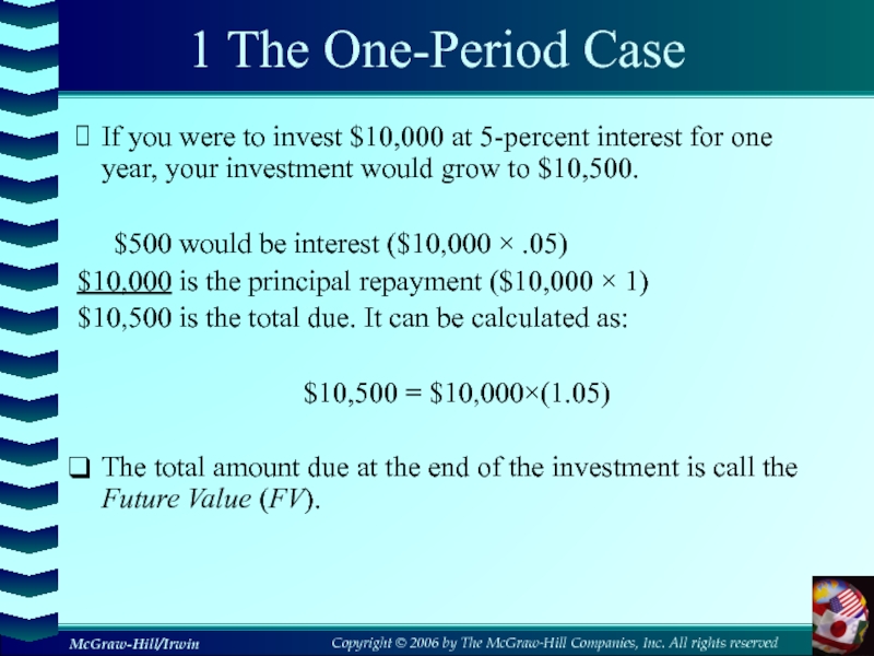
- 6. 1 The One-Period CaseIf you were to
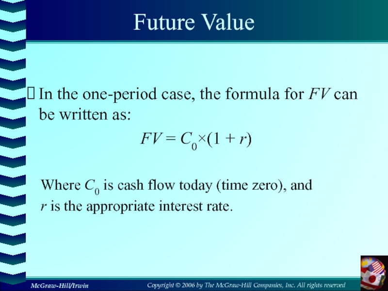
- 7. Future ValueIn the one-period case, the formula
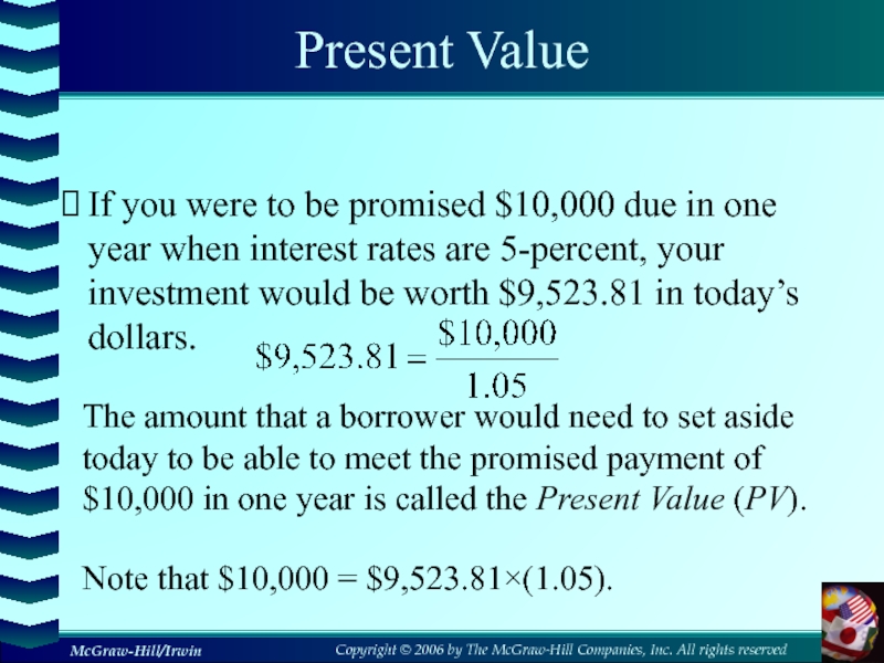
- 8. Present ValueIf you were to be promised
- 9. Present ValueIn the one-period case, the formula
- 10. Net Present ValueThe Net Present Value (NPV)
- 11. Net Present ValueThe present value of the
- 12. Net Present ValueIn the one-period case, the
- 13. 4.2 The Multiperiod CaseThe general formula for
- 14. Future ValueSuppose a stock currently pays a
- 15. Future Value and CompoundingNotice that the dividend
- 16. Future Value and Compounding
- 17. Present Value and DiscountingHow much would an
- 18. Finding the Number of PeriodsIf we deposit
- 19. What Rate Is Enough?Assume the total cost
- 20. Multiple Cash Flows Consider an investment that pays
- 21. Multiple Cash FlowsPresent Value < Cost → Do Not Purchase
- 22. Valuing “Lumpy” Cash FlowsFirst, set your calculator
- 23. 4.3 Compounding PeriodsCompounding an investment m times
- 24. Compounding PeriodsFor example, if you invest $50
- 25. Effective Annual Rates of InterestA reasonable question
- 26. Effective Annual Rates of InterestSo, investing at
- 27. Effective Annual Rates of InterestFind
- 28. EAR on a Financial CalculatorTexas Instruments BAII Plus
- 29. Continuous CompoundingThe general formula for the future
- 30. 4.4 SimplificationsAnnuityA stream of constant cash flows
- 31. AnnuityA constant stream of cash flows with a fixed maturity
- 32. Annuity: ExampleIf you can afford a $400
- 33. What is the present
- 34. Growing AnnuityA growing stream of cash flows with a fixed maturity
- 35. Growing Annuity: ExampleA defined-benefit retirement plan offers
- 36. PerpetuityA constant stream of cash flows that lasts forever…
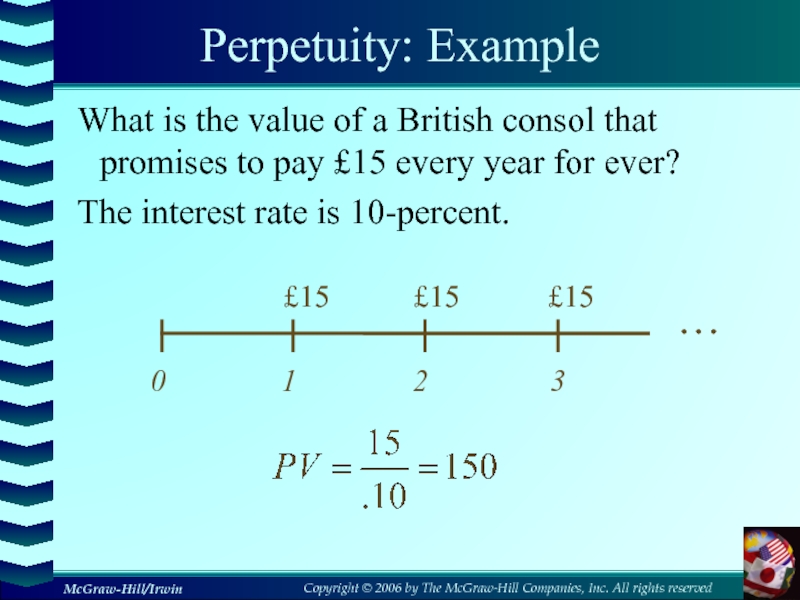
- 37. Perpetuity: ExampleWhat is the value of a
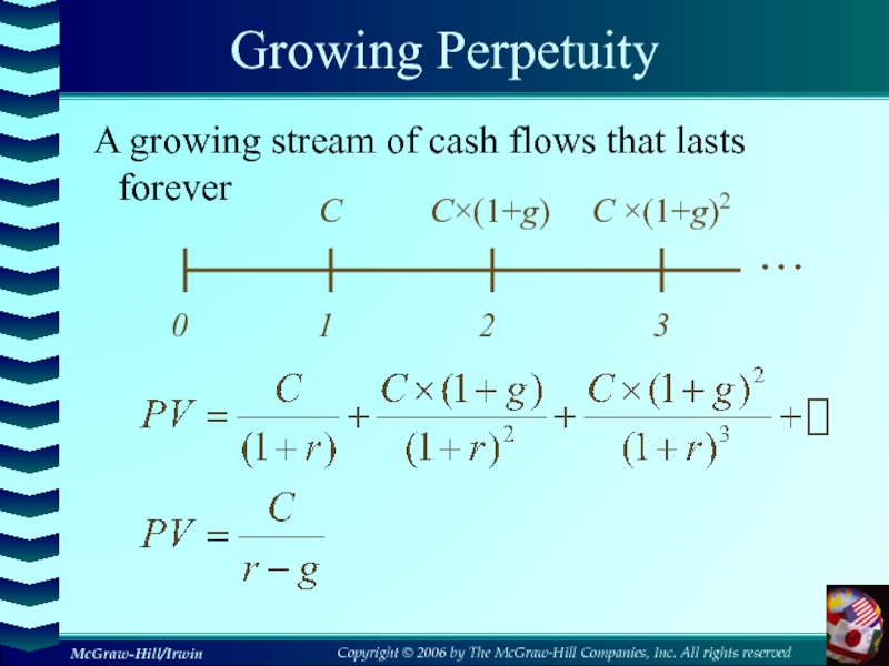
- 38. Growing PerpetuityA growing stream of cash flows that lasts forever…
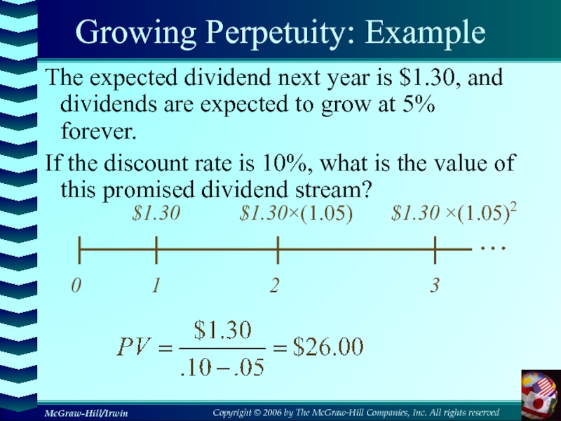
- 39. Growing Perpetuity: ExampleThe expected dividend next year
- 40. Valuation of Bond and StockAfter reviewing the
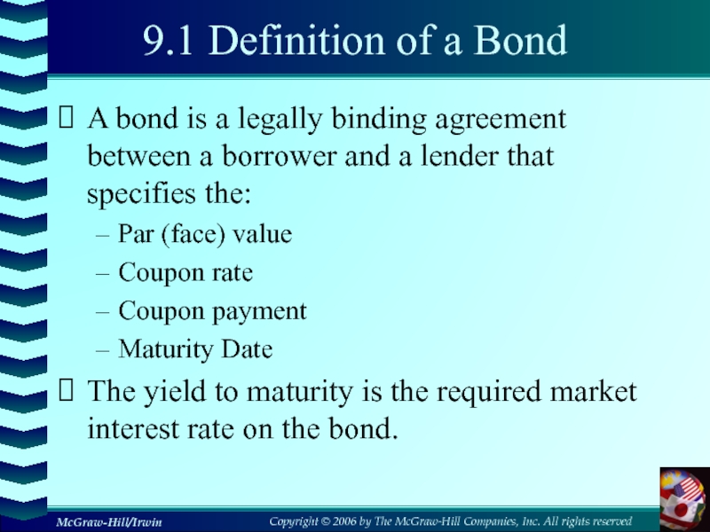
- 41. 9.1 Definition of a BondA bond is
- 42. 9.2 How to Value Bonds Primary Principle:Value
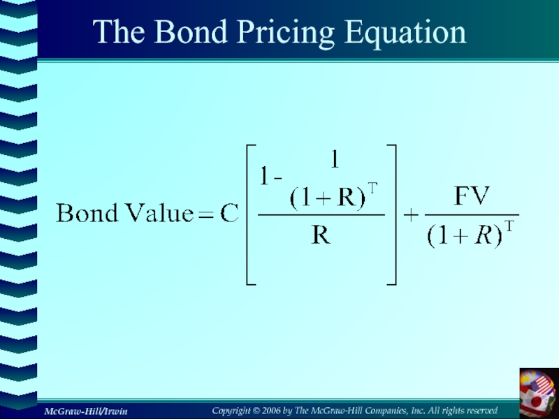
- 43. The Bond Pricing Equation
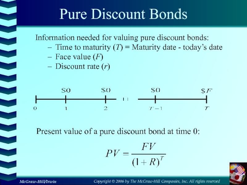
- 44. Pure Discount BondsMake no periodic interest payments
- 45. Pure Discount BondsInformation needed for valuing pure
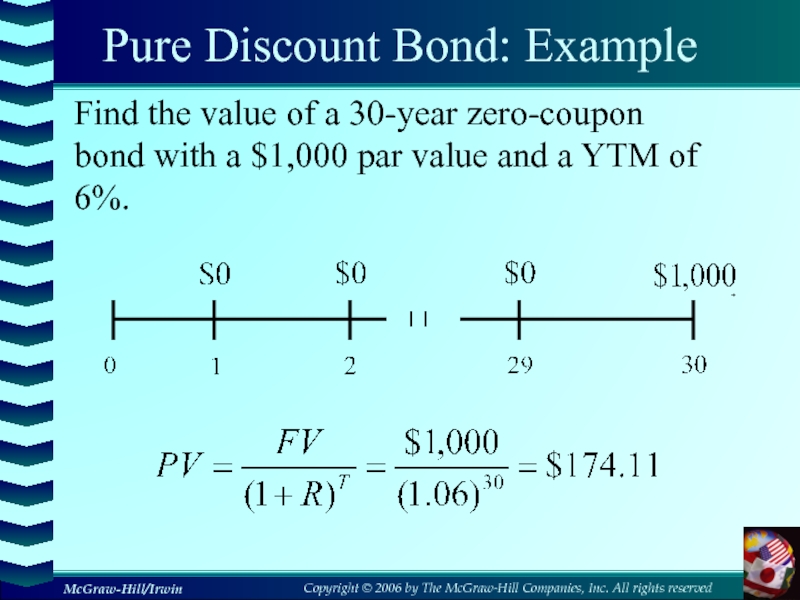
- 46. Pure Discount Bond: ExampleFind the value of
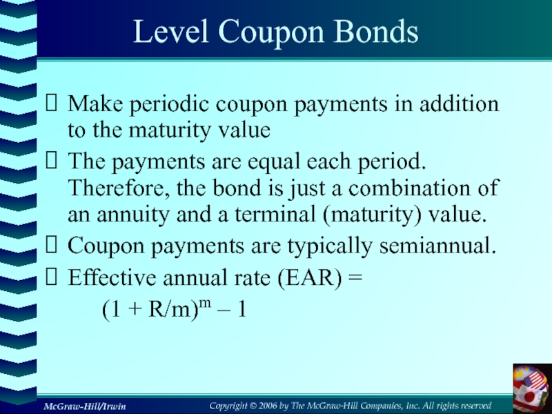
- 47. Level Coupon BondsMake periodic coupon payments in
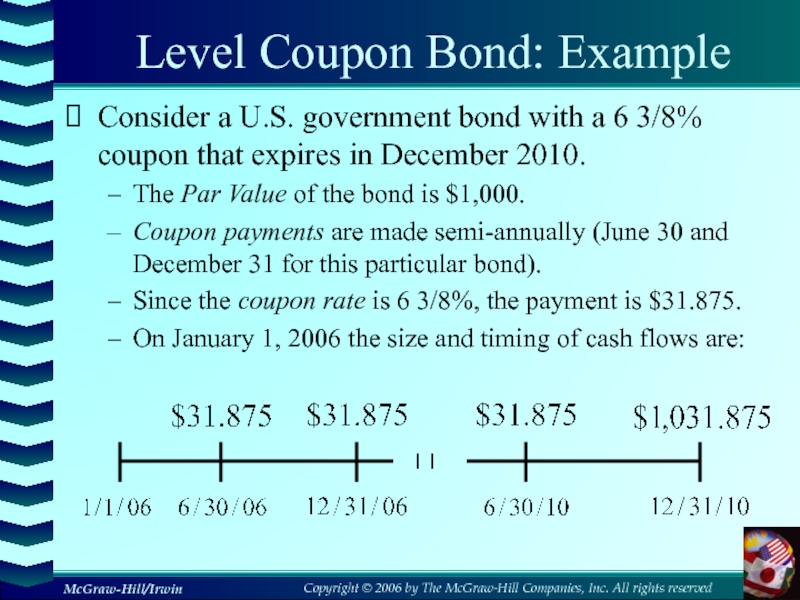
- 48. Level Coupon Bond: ExampleConsider a U.S. government
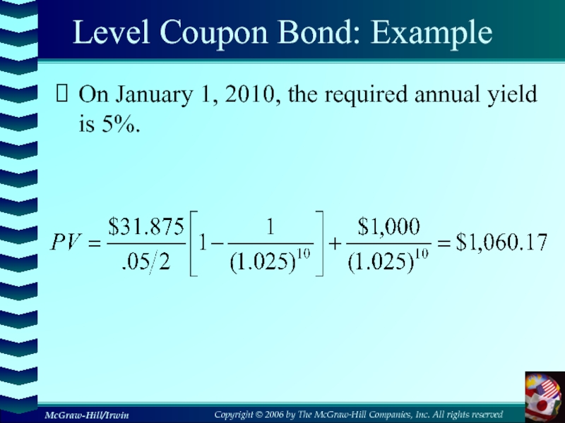
- 49. Level Coupon Bond: ExampleOn January 1, 2010, the required annual yield is 5%.
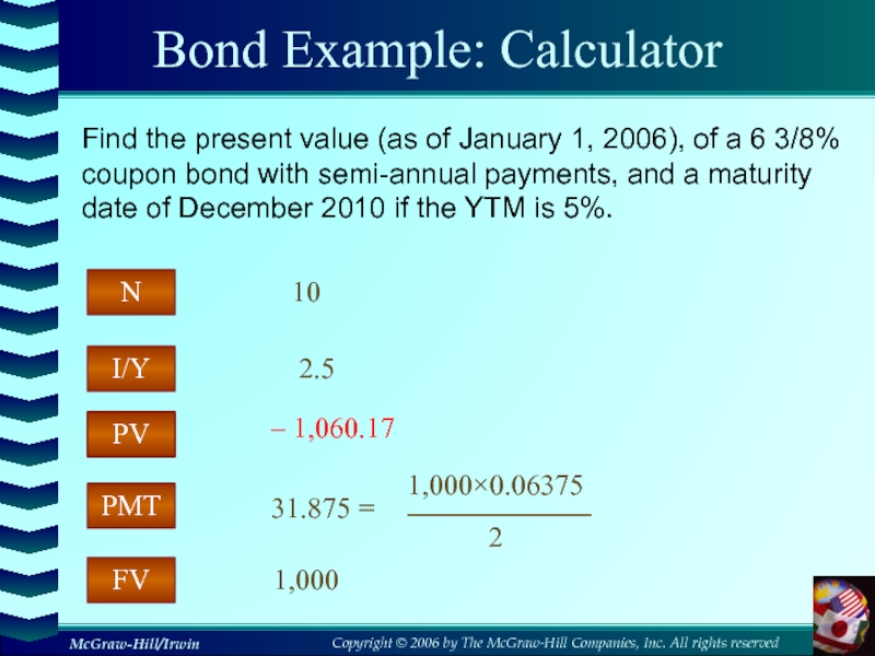
- 50. Bond Example: CalculatorPMTI/YFVPVNPV31.875 =2.51,000– 1,060.1710Find the present
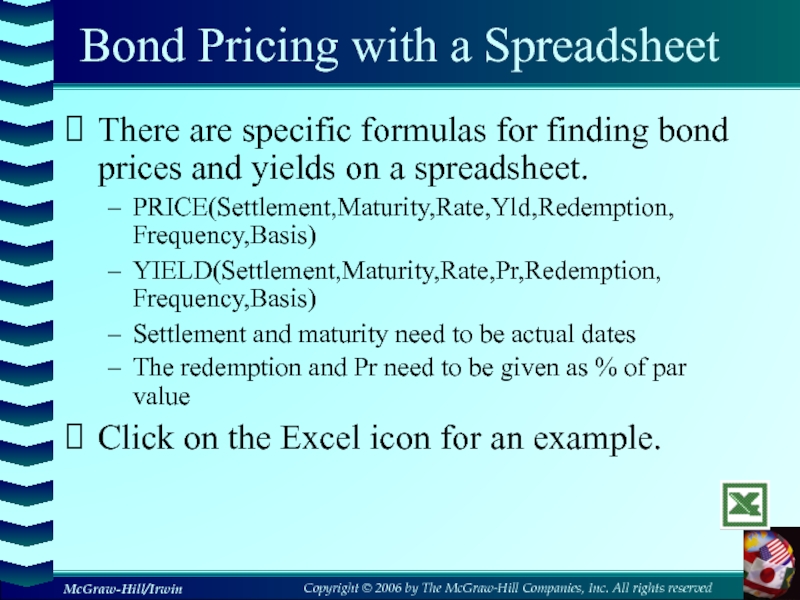
- 51. Bond Pricing with a SpreadsheetThere are specific
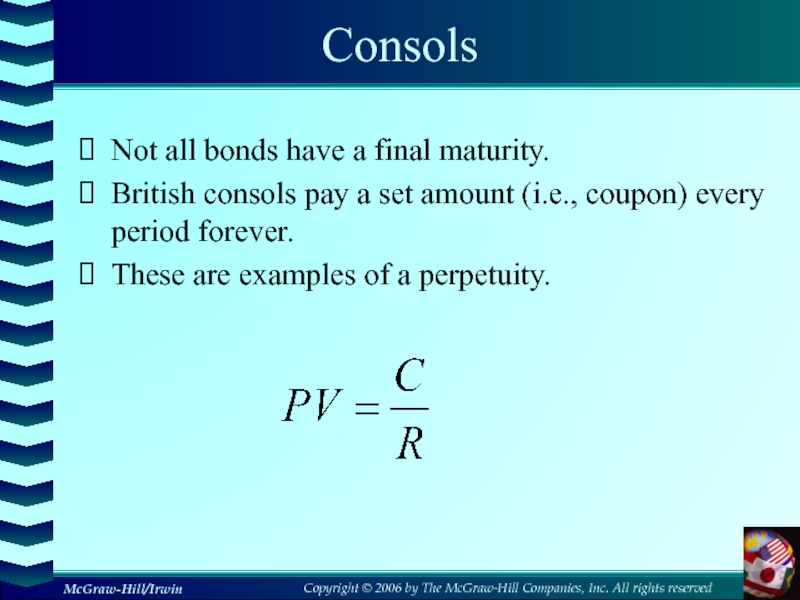
- 52. ConsolsNot all bonds have a final maturity.British
- 53. 9.3 Bond ConceptsBond prices and market interest
- 54. YTM and Bond Value800100011001200130000.010.020.030.040.050.060.070.080.090.1Discount RateBond ValueWhen the
- 55. Bond Example RevisitedUsing our previous example, now
- 56. Computing Yield to MaturityYield to maturity is
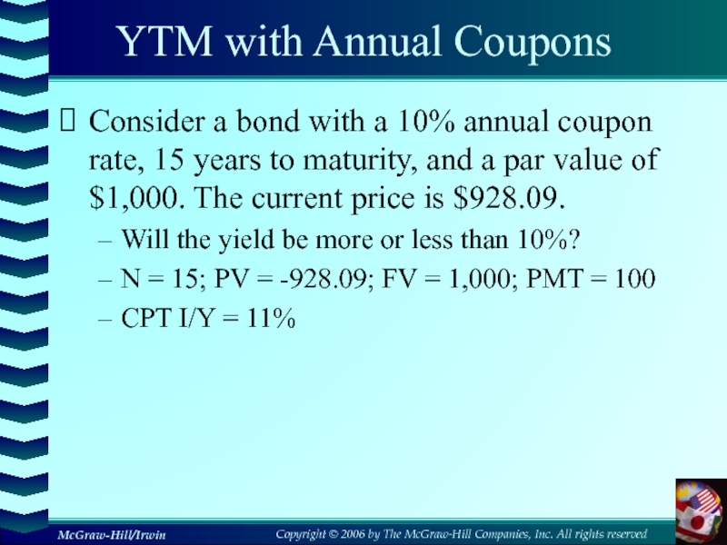
- 57. YTM with Annual CouponsConsider a bond with
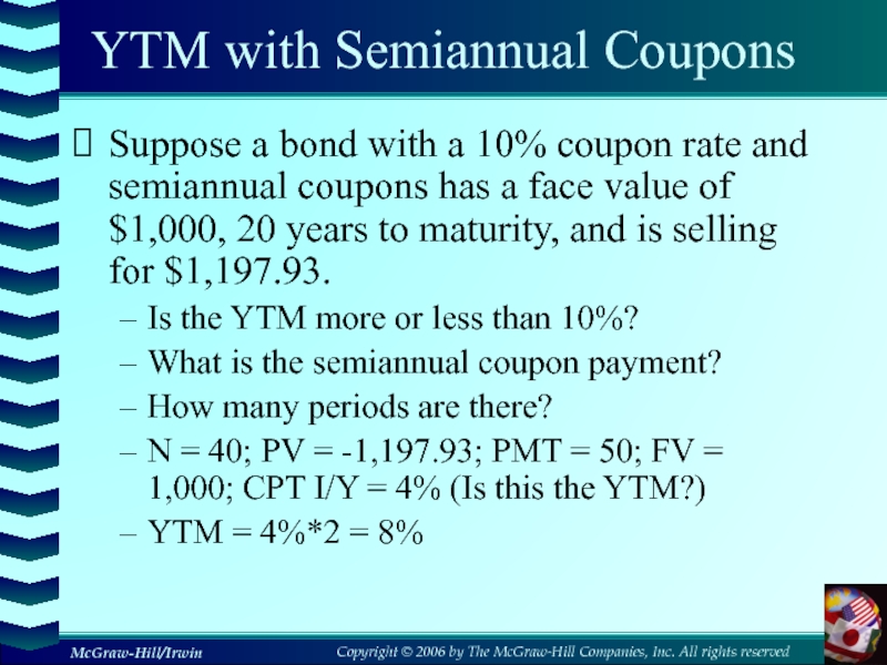
- 58. YTM with Semiannual CouponsSuppose a bond with
- 59. Bond Market ReportingPrimarily over-the-counter transactions with dealers
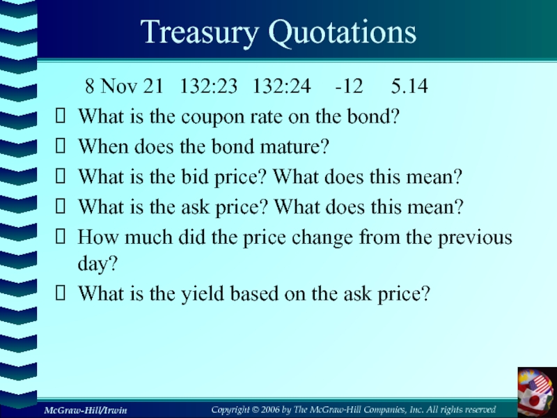
- 60. Treasury Quotations8 Nov 21 132:23 132:24 -12 5.14What is the
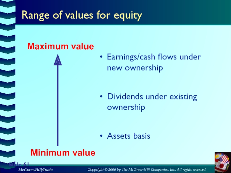
- 61. Slide Range of values for equityEarnings/cash flows under new ownershipDividends under existing ownershipAssets basisMaximum valueMinimum value
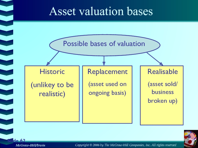
- 62. Slide Asset valuation basesPossible bases of valuationHistoric(unlikey
- 63. Assets basis If a business is
- 64. 9.4 The Present Value of Common StocksThe
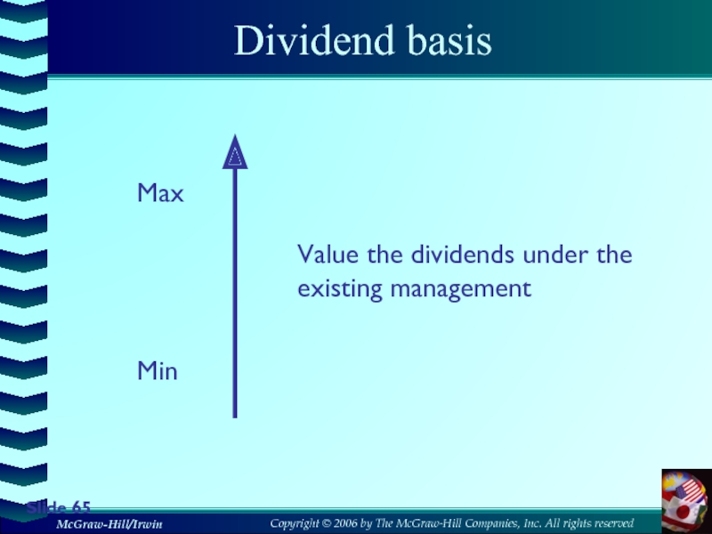
- 65. Dividend basisSlide MaxMinValue the dividends under the existing management
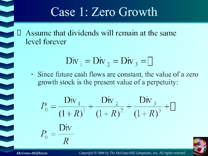
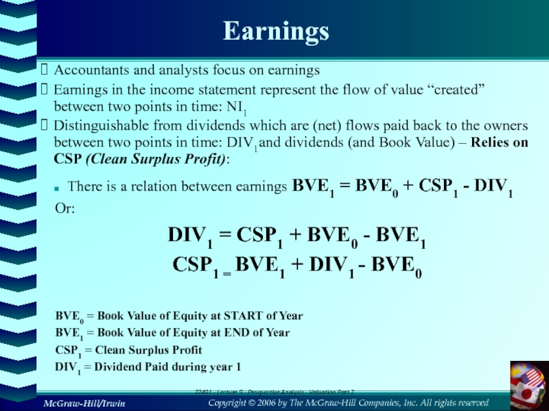
- 66. Case 1: Zero GrowthAssume that dividends will
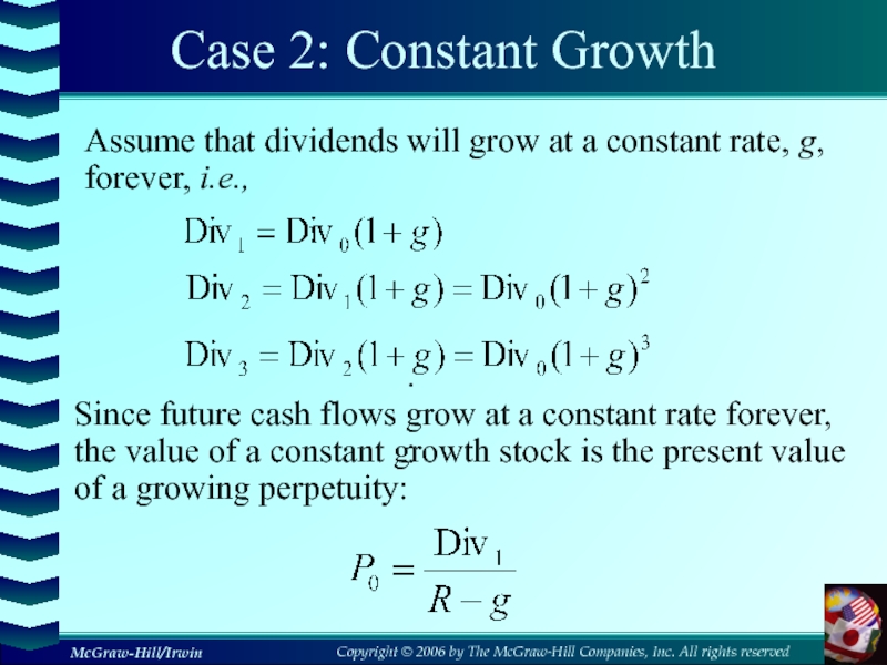
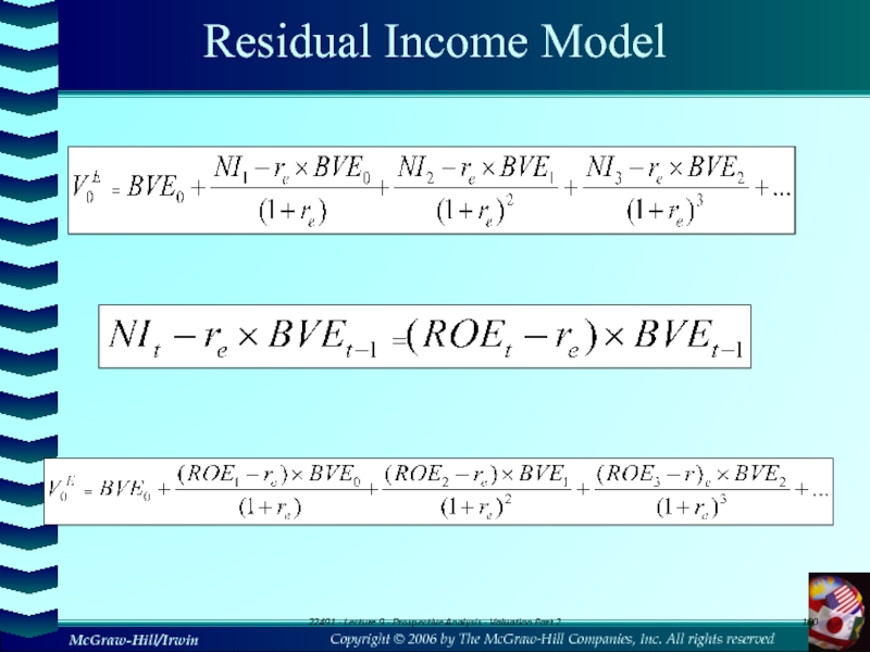
- 67. Case 2: Constant GrowthSince future cash flows
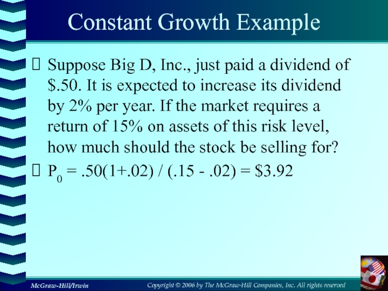
- 68. Constant Growth ExampleSuppose Big D, Inc., just
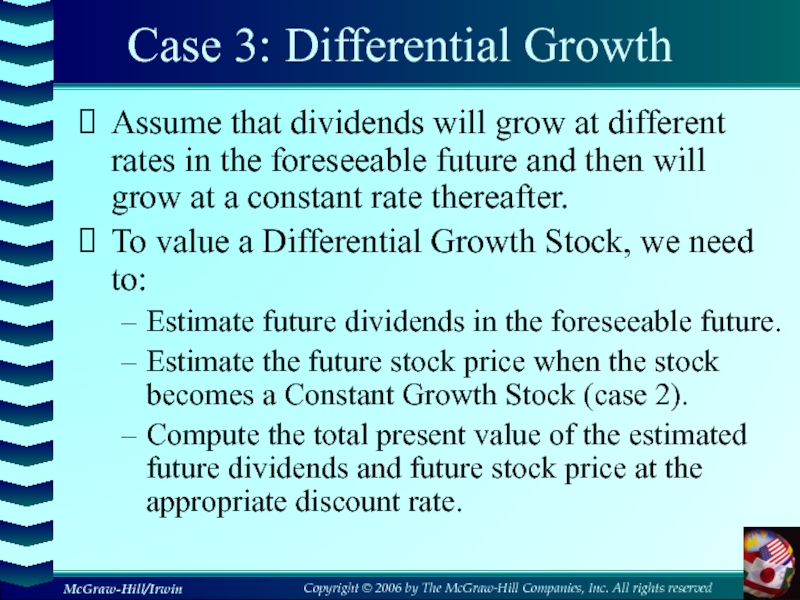
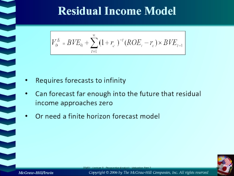
- 69. Case 3: Differential GrowthAssume that dividends will
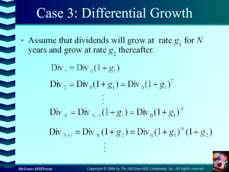
- 70. Case 3: Differential GrowthAssume that dividends will
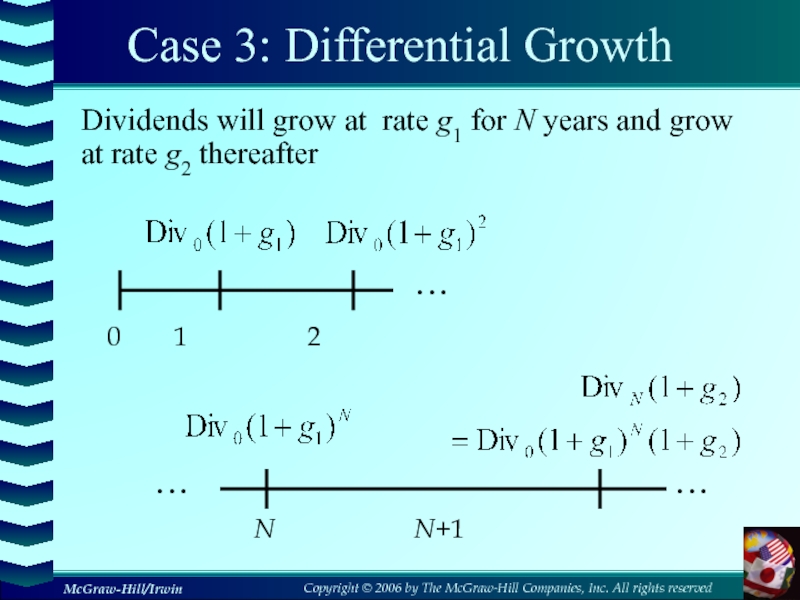
- 71. Case 3: Differential GrowthDividends will grow at
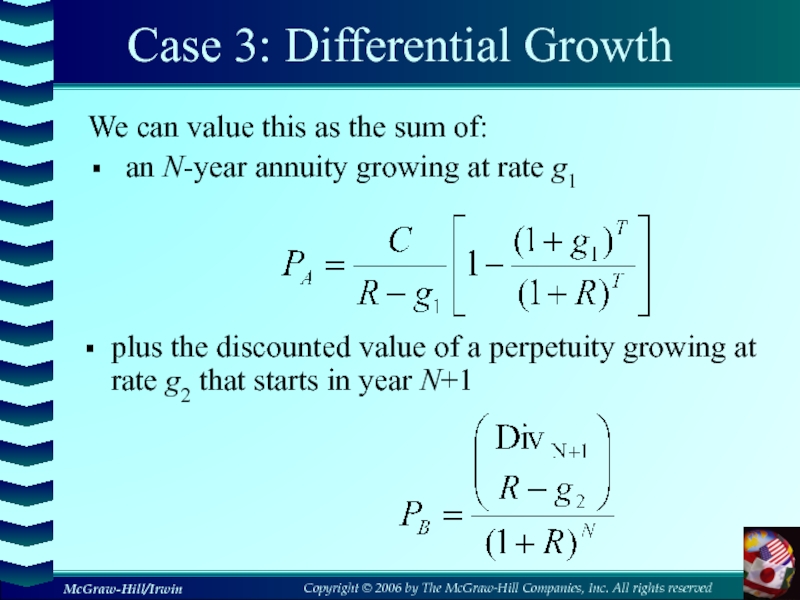
- 72. Case 3: Differential GrowthWe can value this
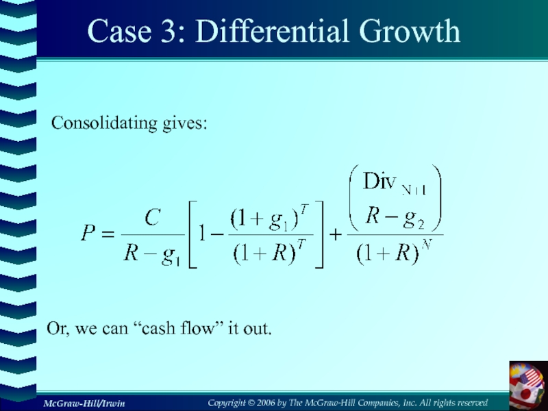
- 73. Case 3: Differential GrowthConsolidating gives:Or, we can “cash flow” it out.
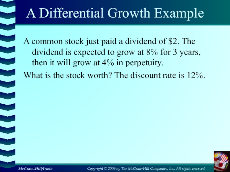
- 74. A Differential Growth ExampleA common stock just
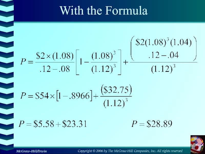
- 75. With the Formula
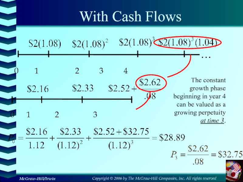
- 76. With Cash Flows…0 1
- 77. DisadvantagesSlide It is difficult to estimating future
- 78. The Red Bud Co. just paid a
- 79. 9.5 Estimates of ParametersThe value of a
- 80. Where does R come from?The discount rate
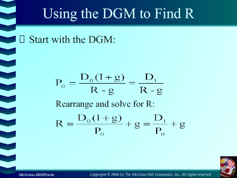
- 81. Using the DGM to Find RStart with the DGM:Rearrange and solve for R:
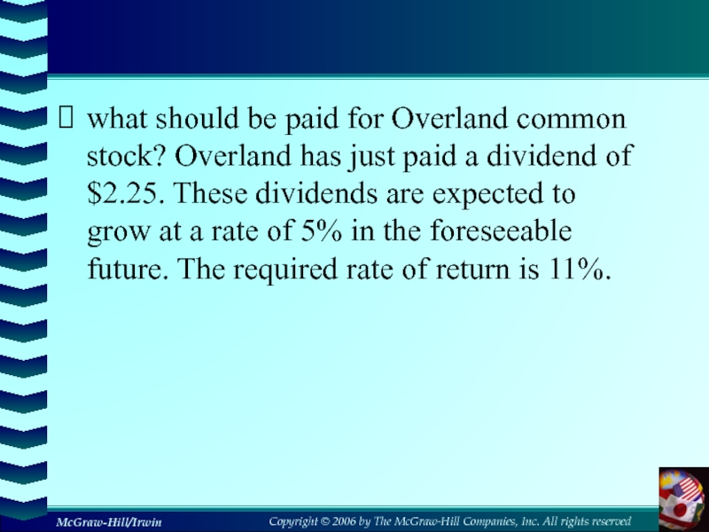
- 82. what should be paid for Overland common
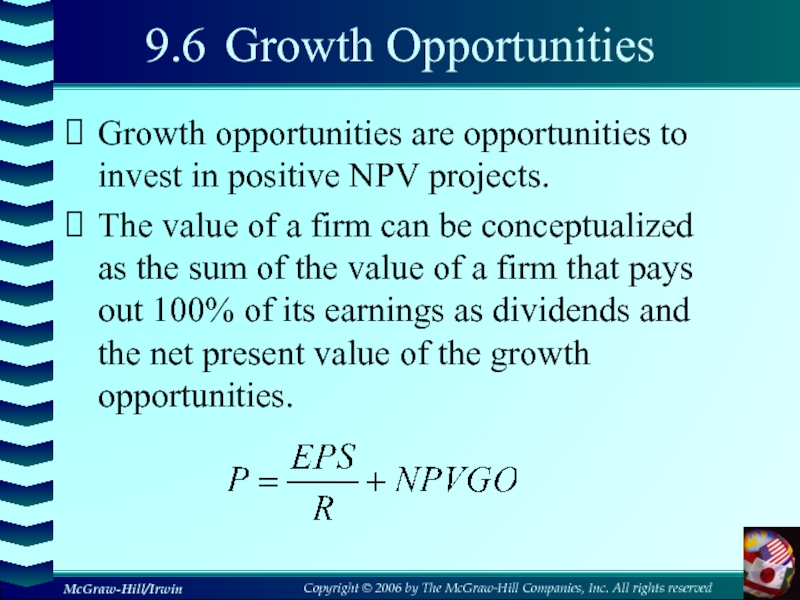
- 83. 9.6 Growth OpportunitiesGrowth opportunities are opportunities to invest
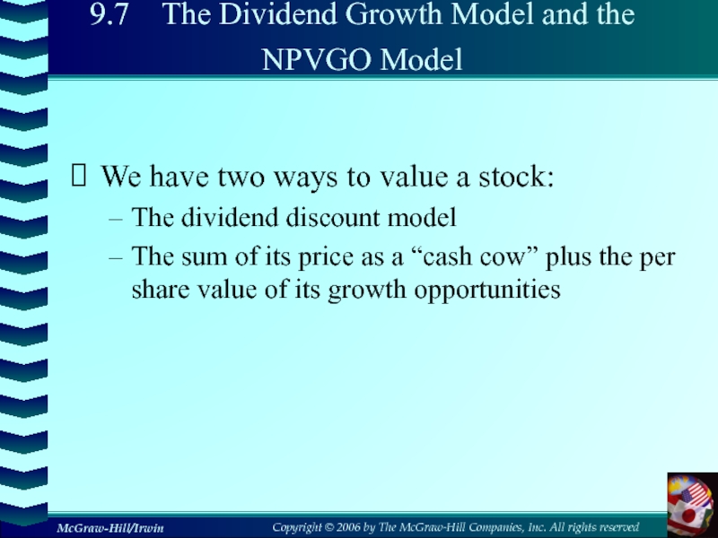
- 84. 9.7 The Dividend Growth Model and the NPVGO
- 85. The NPVGO Model: Example Consider a
- 86. The NPVGO Model: Example First, we
- 87. 9.8 Price-Earnings RatioMany analysts frequently relate earnings per
- 88. 9.9 Stock Market Reporting
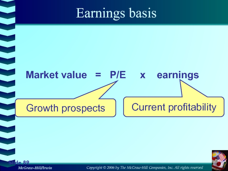
- 89. Slide Earnings basisMarket value = P/E x earningsGrowth prospectsCurrent profitability
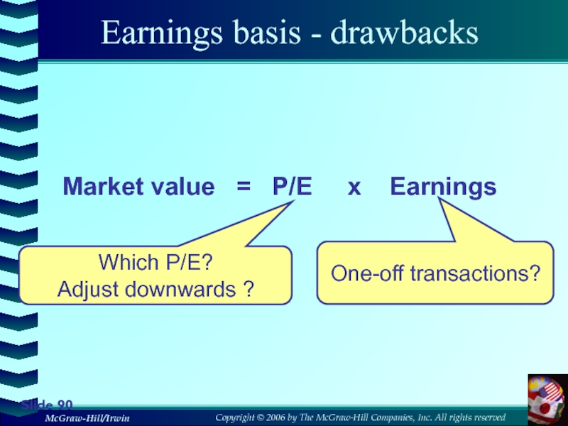
- 90. Slide Earnings basis - drawbacksMarket value
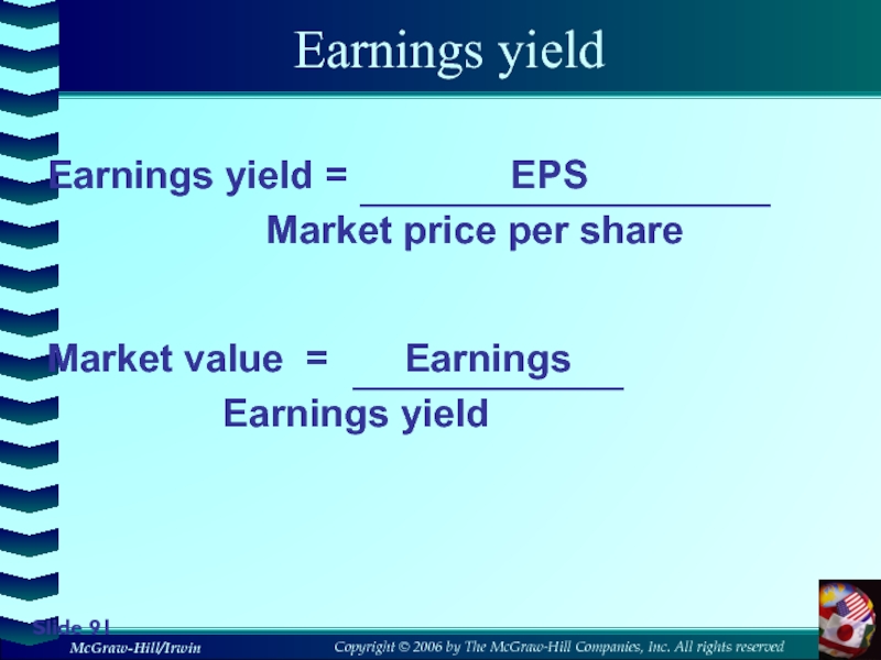
- 91. Slide Earnings yieldMarket value =
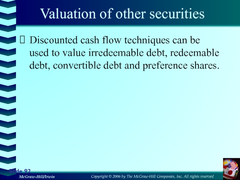
- 92. Valuation of other securitiesDiscounted cash flow techniques
- 93. Quick QuizHow do you find the value
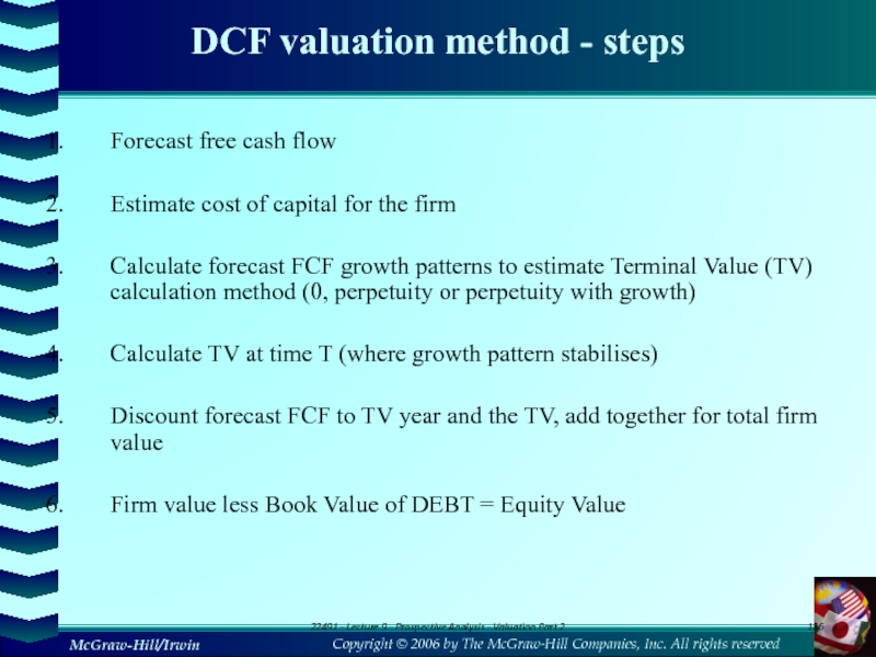
- 94. Lecture 9Prospective Analysis – Valuation theory and
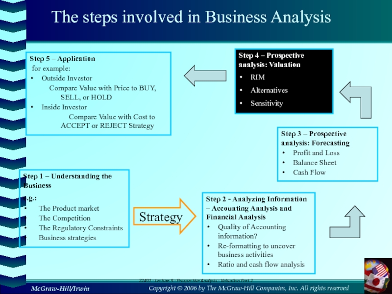
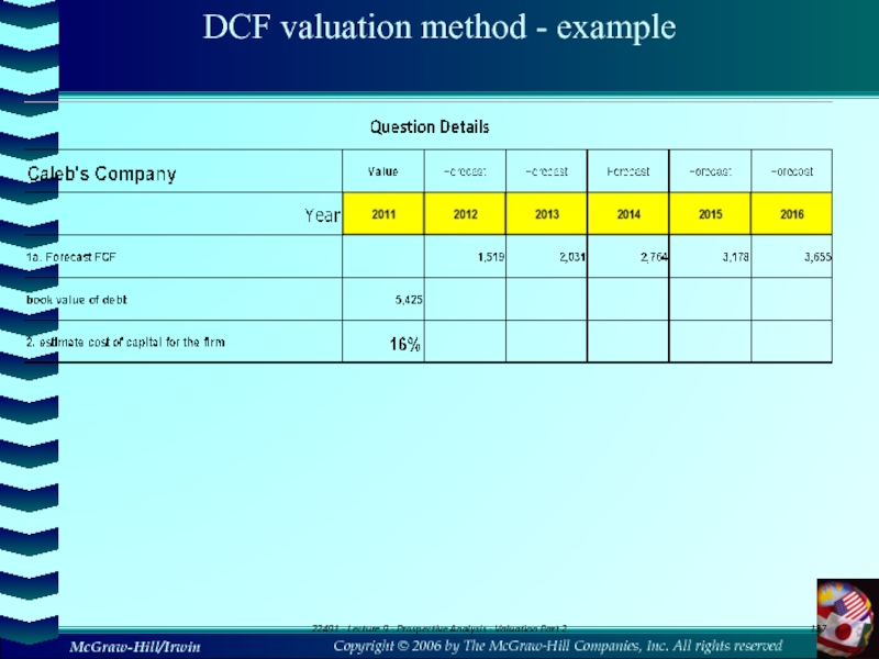
- 95. The steps involved in Business AnalysisStep 1
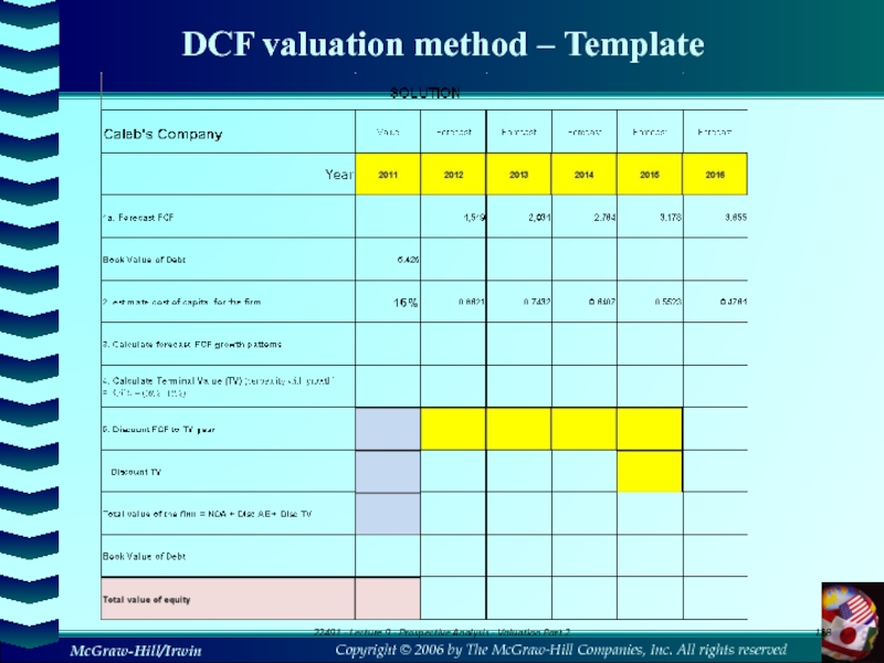
- 96. Learning ObjectivesAt the conclusion of this lecture
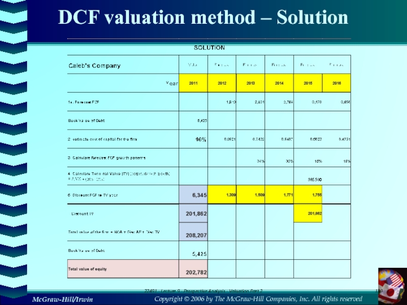
- 97. ValuationIs the process of converting the forecast
- 98. EarningsAccountants and analysts focus on earningsEarnings in
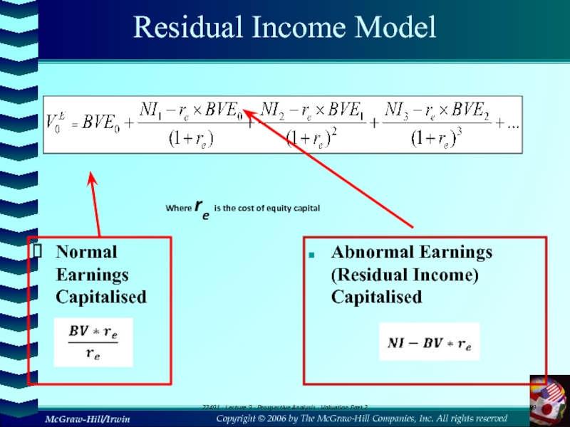
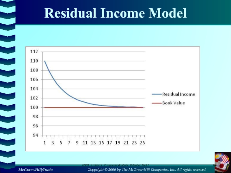
- 99. Residual Income ModelNormal Earnings Capitalised Abnormal Earnings (Residual
- 100. Residual Income Model22491 - Lecture 9 - Prospective Analysis - Valuation Part 2
- 101. Residual Income ModelRequires forecasts to infinityCan forecast
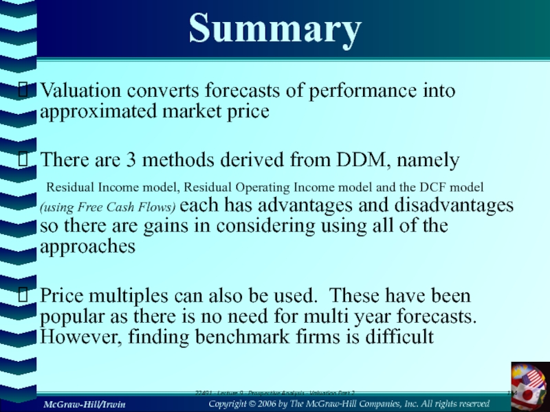
- 102. Residual Income Model22491 - Lecture 9 - Prospective Analysis - Valuation Part 2
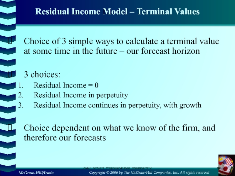
- 103. Residual Income Model – Terminal ValuesChoice of
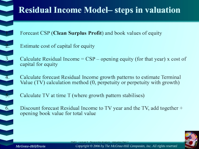
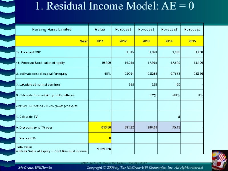
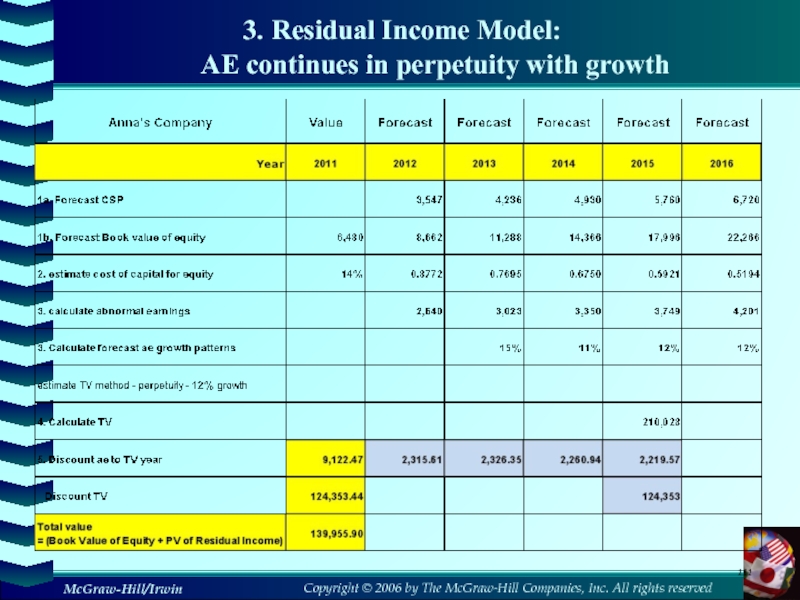
- 104. Residual Income Model– steps in valuationForecast CSP
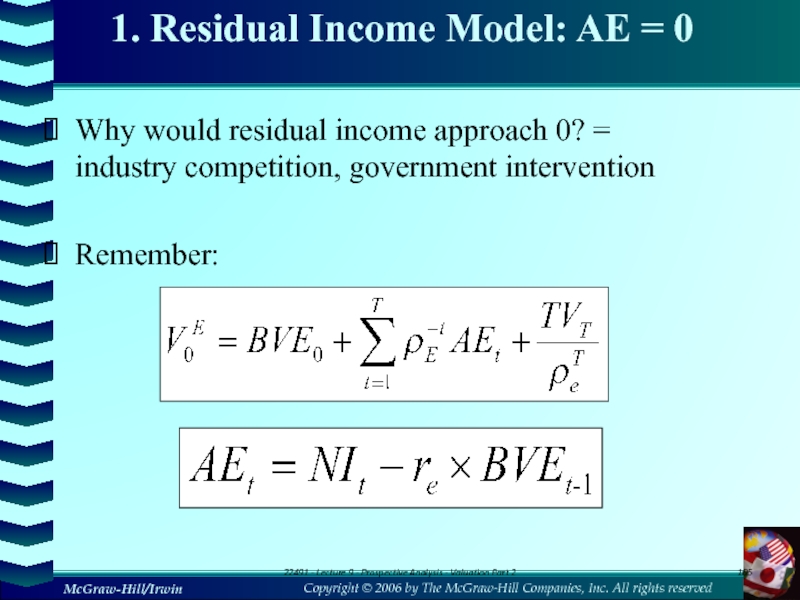
- 105. 1. Residual Income Model: AE = 0Why
- 106. 1. Residual Income Model: AE = 022491
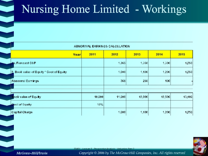
- 107. Nursing Home Limited - Workings22491 - Lecture 9 - Prospective Analysis - Valuation Part 2
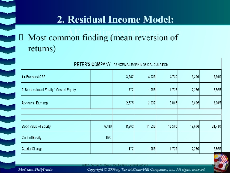
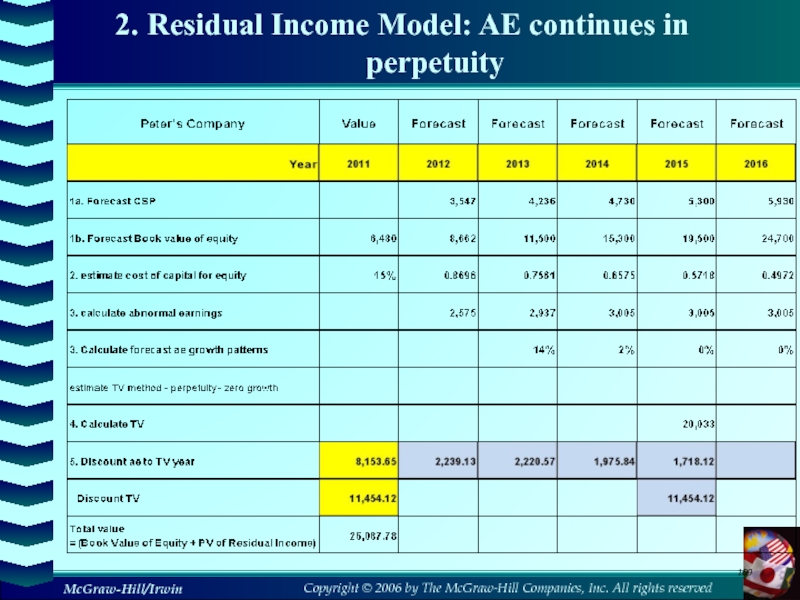
- 108. 2. Residual Income Model: AE continues
- 109. 2. Residual Income Model: AE continues in perpetuity
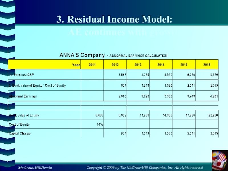
- 110. 3. Residual Income Model: AE continues with growth
- 111. 3. Residual Income Model: AE continues in perpetuity with growth
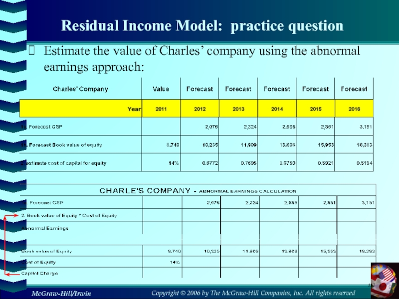
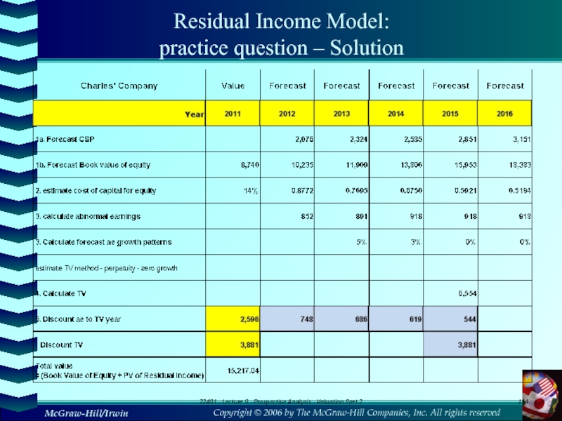
- 112. Residual Income Model: practice questionEstimate the value of Charles’ company using the abnormal earnings approach:
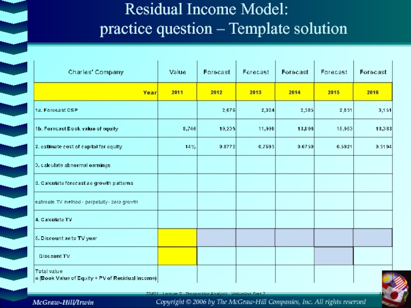
- 113. Residual Income Model: practice question –
- 114. Residual Income Model: practice question –
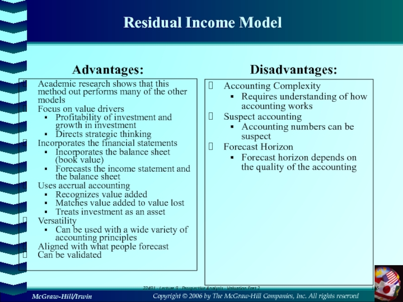
- 115. Residual Income ModelAdvantages:Academic research shows that this
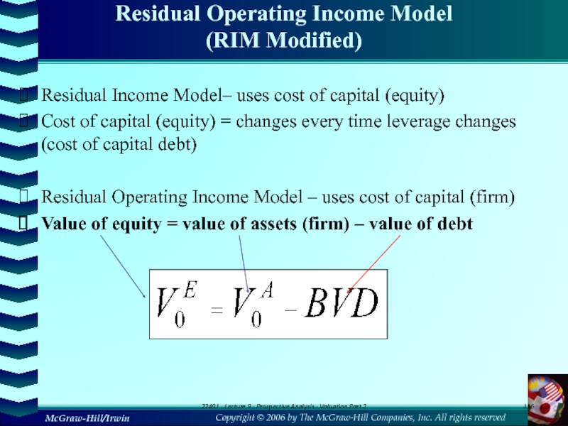
- 116. Residual Operating Income Model (RIM Modified)Residual
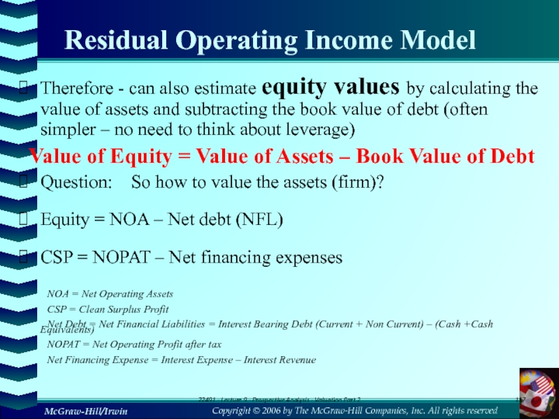
- 117. Residual Operating Income ModelTherefore - can also
- 118. Residual OPERATING Income ModelUnder the discounted abnormal
- 119. Residual Operating Income ModelGives the same result
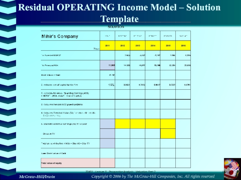
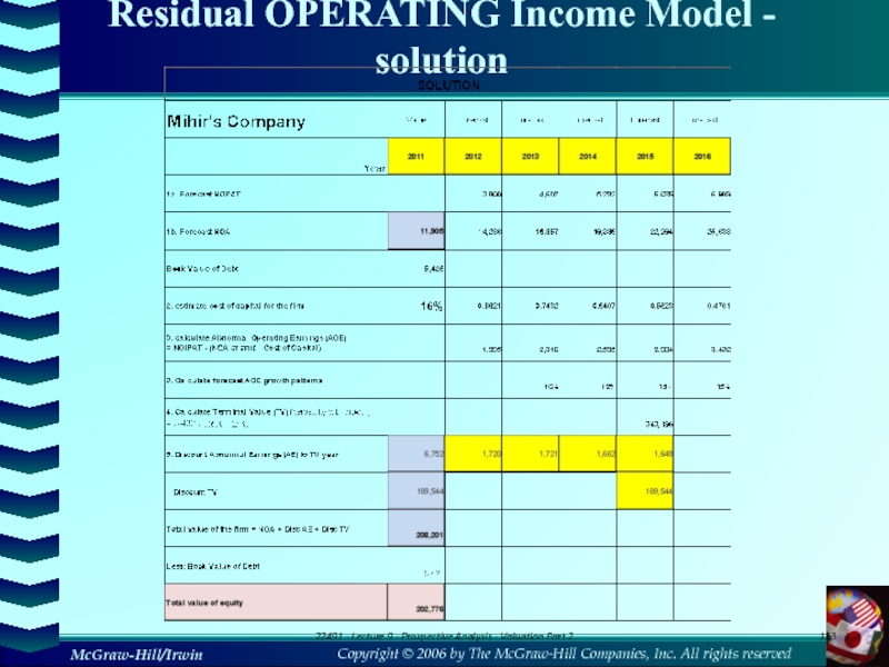
- 120. Residual Operating Income Model - stepsForecast NOPAT
- 121. Residual Operating Income Model - questionEstimate the
- 122. Residual OPERATING Income Model – Solution Template22491
- 123. Residual OPERATING Income Model - solution22491 - Lecture 9 - Prospective Analysis - Valuation Part 2
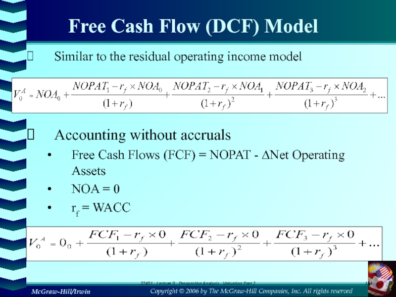
- 124. Free Cash Flow (DCF) ModelSimilar to the
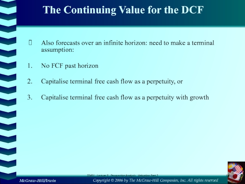
- 125. Also forecasts over an infinite horizon: need
- 126. DCF valuation method - stepsForecast free cash
- 127. DCF valuation method - example22491 - Lecture 9 - Prospective Analysis - Valuation Part 2
- 128. DCF valuation method – Template22491 - Lecture 9 - Prospective Analysis - Valuation Part 2
- 129. DCF valuation method – Solution22491 - Lecture 9 - Prospective Analysis - Valuation Part 2
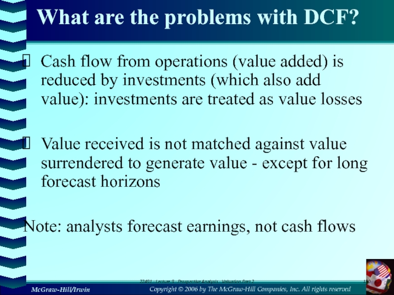
- 130. What are the problems with DCF?Cash flow
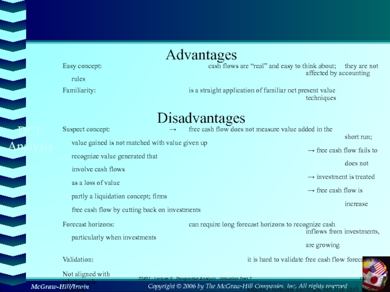
- 131. DCF AnalysisAdvantagesEasy concept: cash flows are “real” and
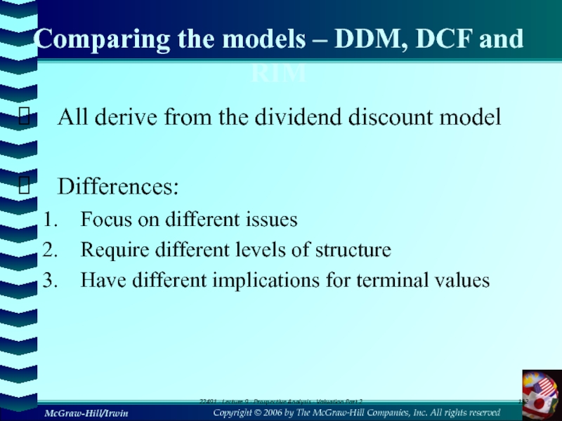
- 132. Comparing the models – DDM, DCF and
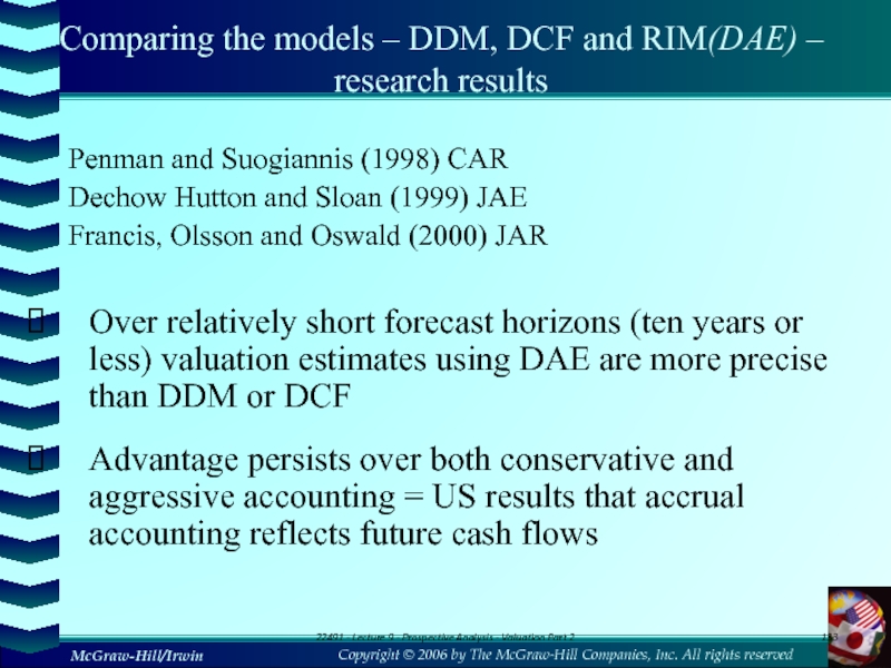
- 133. Comparing the models – DDM, DCF and
- 134. SummaryValuation converts forecasts of performance into approximated
- 135. Скачать презентанцию
Слайды и текст этой презентации
Слайд 1Chapter 9
Corporate Finance
Value of Bond and Common Stocks
Copyright © 2006
by The McGraw-Hill Companies, Inc. All rights reserved
Слайд 2Key Concepts and Skills
Know the important bond features and bond
types
Understand bond values and why they fluctuate
Understand how stock prices
depend on future dividends and dividend growthBe able to compute stock prices using the dividend growth model
Understand how growth opportunities affect stock values
Слайд 3Chapter Outline
9.1 Definitions and Example of a Bond
9.2 How to Value Bonds
9.3 Bond
Concepts
9.4 The Present Value of Common Stocks
9.5 Estimates of Parameters in the
Dividend- Discount Model9.6 Growth Opportunities
9.7 The Dividend Growth Model and the NPVGO Model
9.8 Price-Earnings Ratio
9.9 Stock Market Reporting
Слайд 4Slide
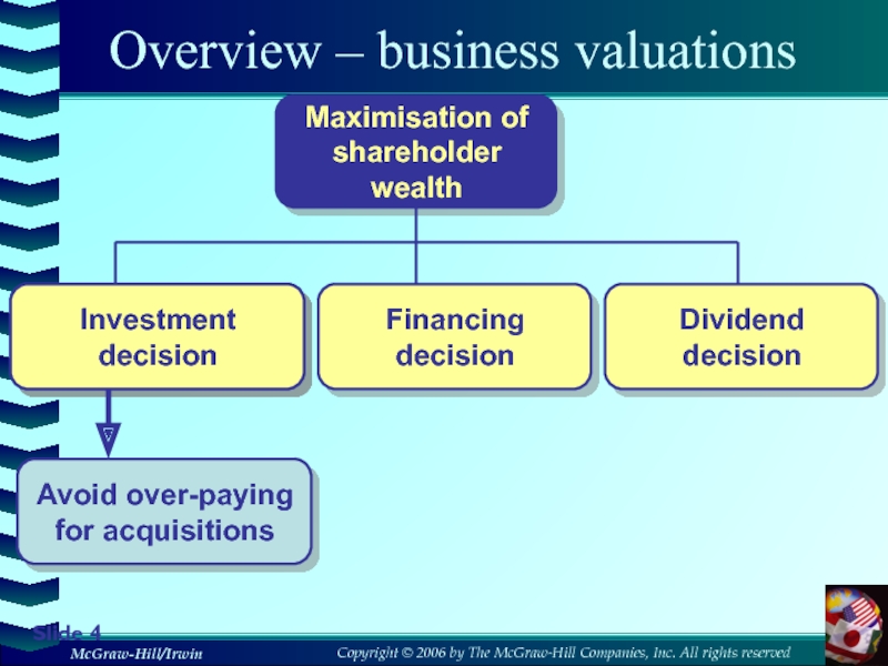
Overview – business valuations
Maximisation of
shareholder wealth
Investment decision
Avoid over-paying
for
acquisitions
Слайд 5Review :Time Value
1 Valuation: The One-Period Case
2 The Multiperiod Case
3
Compounding Periods
4 Simplifications
6 What Is a Firm Worth?
Слайд 61 The One-Period Case
If you were to invest $10,000 at
5-percent interest for one year, your investment would grow to
$10,500.$500 would be interest ($10,000 × .05)
$10,000 is the principal repayment ($10,000 × 1)
$10,500 is the total due. It can be calculated as:
$10,500 = $10,000×(1.05)
The total amount due at the end of the investment is call the Future Value (FV).
Слайд 7Future Value
In the one-period case, the formula for FV can
be written as:
FV = C0×(1 + r)
Where C0 is cash
flow today (time zero), and r is the appropriate interest rate.
Слайд 8Present Value
If you were to be promised $10,000 due in
one year when interest rates are 5-percent, your investment would
be worth $9,523.81 in today’s dollars.The amount that a borrower would need to set aside today to be able to meet the promised payment of $10,000 in one year is called the Present Value (PV).
Note that $10,000 = $9,523.81×(1.05).
Слайд 9Present Value
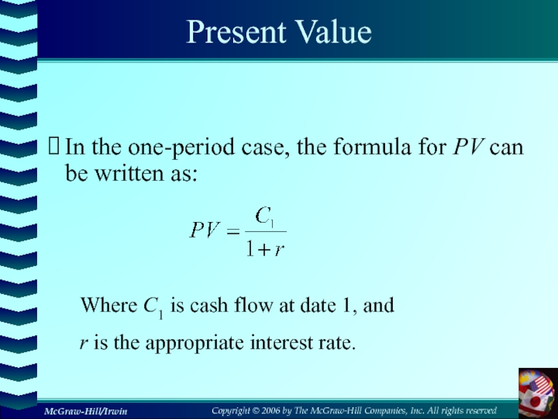
In the one-period case, the formula for PV can
be written as:
Where C1 is cash flow at date 1,
and r is the appropriate interest rate.
Слайд 10Net Present Value
The Net Present Value (NPV) of an investment
is the present value of the expected cash flows, less
the cost of the investment.Suppose an investment that promises to pay $10,000 in one year is offered for sale for $9,500. Your interest rate is 5%. Should you buy?
Слайд 11Net Present Value
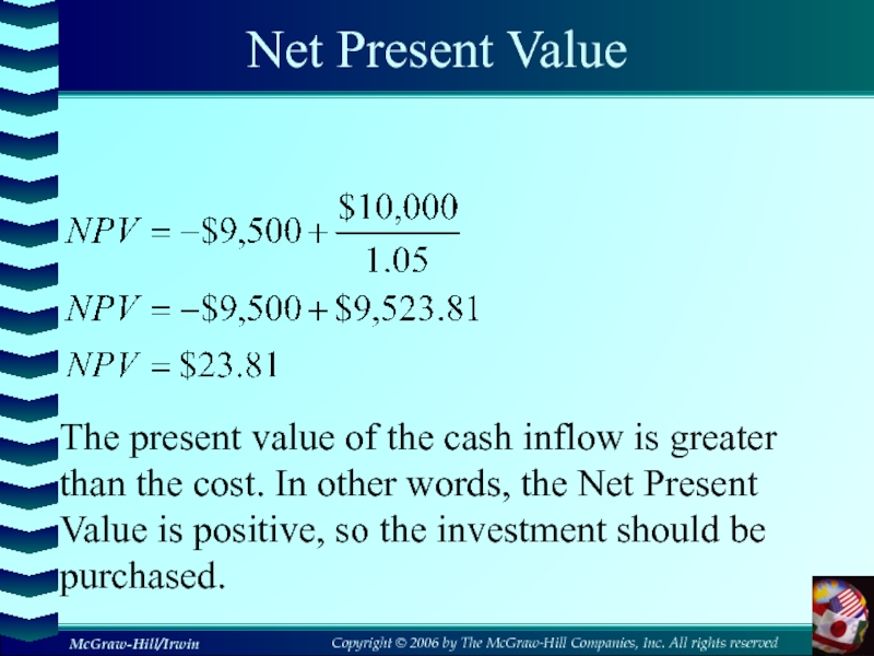
The present value of the cash inflow is
greater
than the cost. In other words, the Net Present
Value is
positive, so the investment should be purchased.
Слайд 12Net Present Value
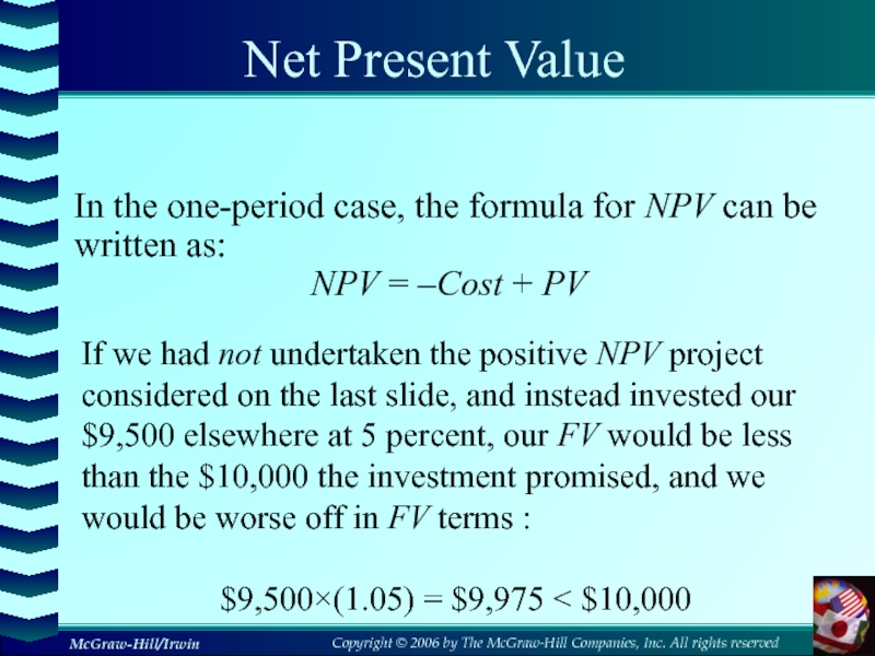
In the one-period case, the formula for NPV
can be written as:
NPV = –Cost + PV
If we had
not undertaken the positive NPV project considered on the last slide, and instead invested our $9,500 elsewhere at 5 percent, our FV would be less than the $10,000 the investment promised, and we would be worse off in FV terms :$9,500×(1.05) = $9,975 < $10,000
Слайд 134.2 The Multiperiod Case
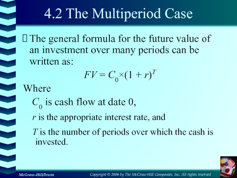
The general formula for the future value
of an investment over many periods can be written as:
FV
= C0×(1 + r)TWhere
C0 is cash flow at date 0,
r is the appropriate interest rate, and
T is the number of periods over which the cash is invested.
Слайд 14Future Value
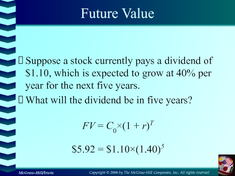
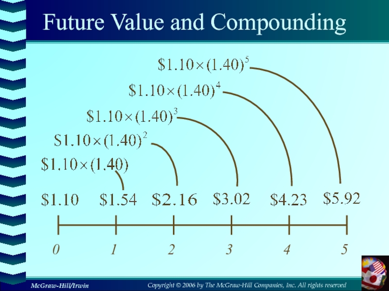
Suppose a stock currently pays a dividend of $1.10,
which is expected to grow at 40% per year for
the next five years.What will the dividend be in five years?
FV = C0×(1 + r)T
$5.92 = $1.10×(1.40)5
Слайд 15Future Value and Compounding
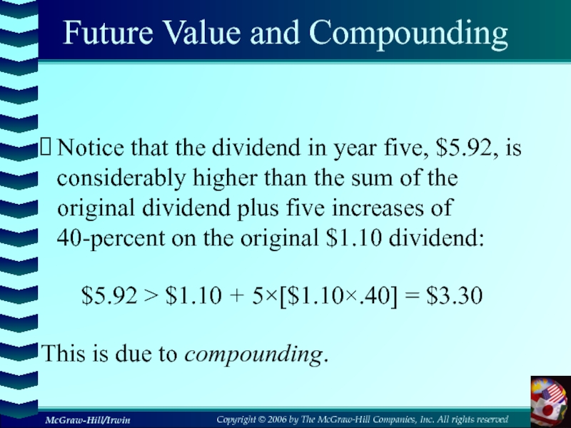
Notice that the dividend in year five,
$5.92, is considerably higher than the sum of the original
dividend plus five increases of 40-percent on the original $1.10 dividend:$5.92 > $1.10 + 5×[$1.10×.40] = $3.30
This is due to compounding.
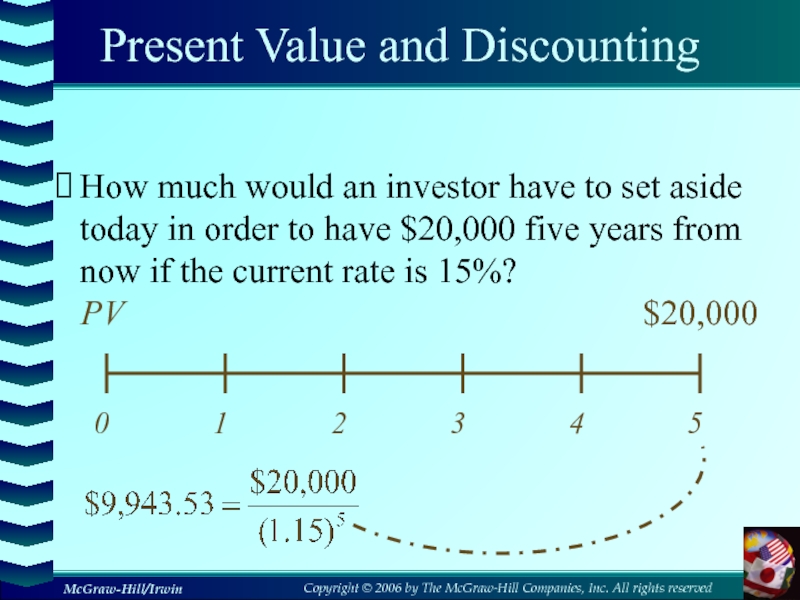
Слайд 17Present Value and Discounting
How much would an investor have to
set aside today in order to have $20,000 five years
from now if the current rate is 15%?$20,000
PV
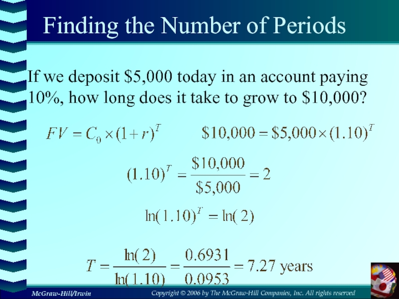
Слайд 18Finding the Number of Periods
If we deposit $5,000 today in
an account paying 10%, how long does it take to
grow to $10,000?Слайд 19What Rate Is Enough?
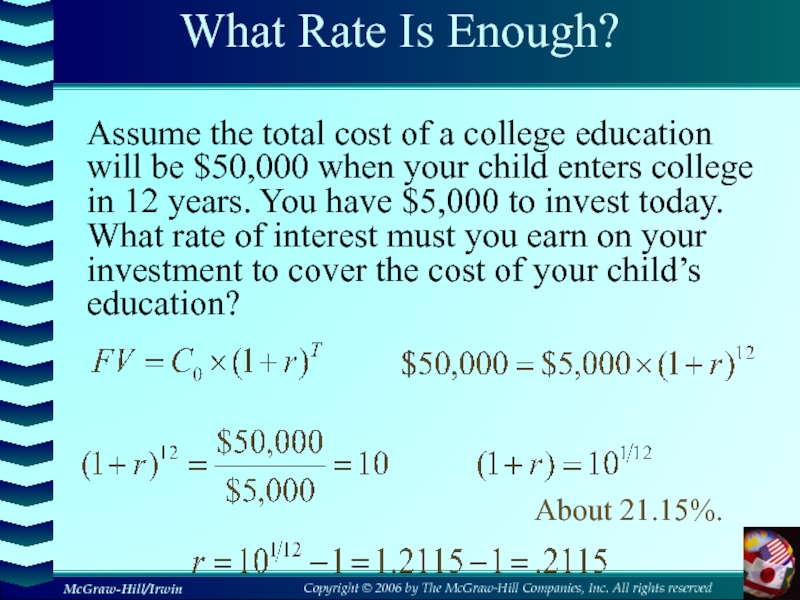
Assume the total cost of a college
education will be $50,000 when your child enters college in
12 years. You have $5,000 to invest today. What rate of interest must you earn on your investment to cover the cost of your child’s education?About 21.15%.
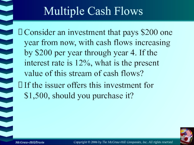
Слайд 20Multiple Cash Flows
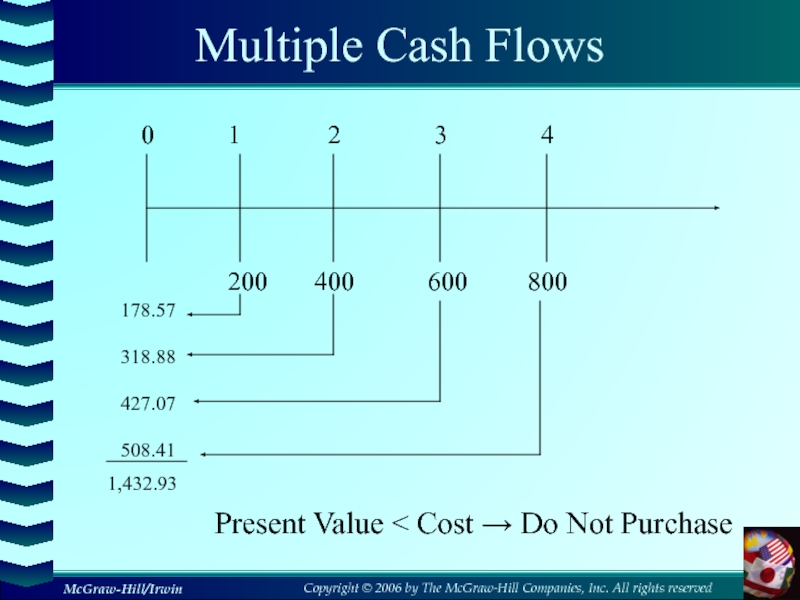
Consider an investment that pays $200 one year
from now, with cash flows increasing by $200 per year
through year 4. If the interest rate is 12%, what is the present value of this stream of cash flows?If the issuer offers this investment for $1,500, should you purchase it?
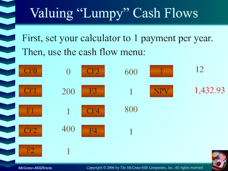
Слайд 22Valuing “Lumpy” Cash Flows
First, set your calculator to 1 payment
per year.
Then, use the cash flow menu:
CF2
CF1
F2
F1
CF0
1
200
1
1,432.93
0
400
I
NPV
12
CF4
CF3
F4
F3
1
600
1
800
Слайд 234.3 Compounding Periods
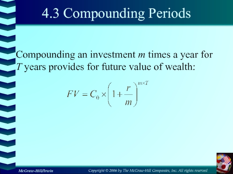
Compounding an investment m times a year for
T years provides for future value of wealth:
Слайд 24Compounding Periods
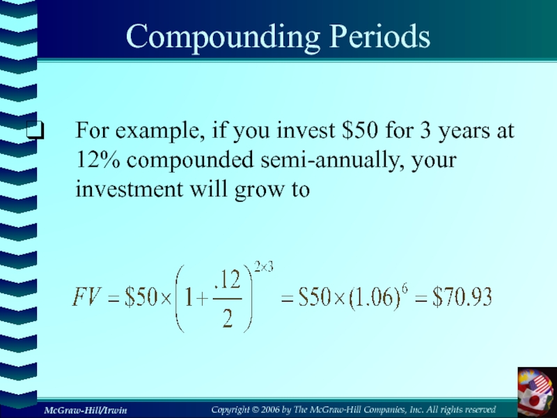
For example, if you invest $50 for 3 years
at 12% compounded semi-annually, your investment will grow to
Слайд 25Effective Annual Rates of Interest
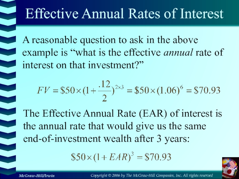
A reasonable question to ask in
the above example is “what is the effective annual rate
of interest on that investment?”The Effective Annual Rate (EAR) of interest is the annual rate that would give us the same end-of-investment wealth after 3 years:
Слайд 26Effective Annual Rates of Interest
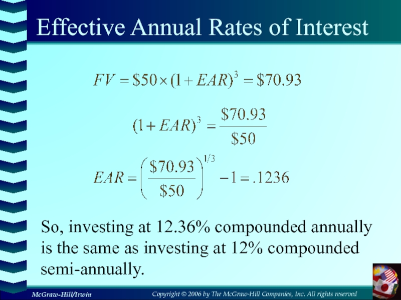
So, investing at 12.36% compounded annually
is the same as investing at 12% compounded semi-annually.
Слайд 27 Effective Annual Rates of Interest
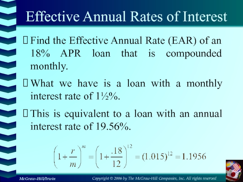
Find the Effective Annual
Rate (EAR) of an 18% APR loan that is compounded
monthly.What we have is a loan with a monthly interest rate of 1½%.
This is equivalent to a loan with an annual interest rate of 19.56%.
Слайд 29Continuous Compounding
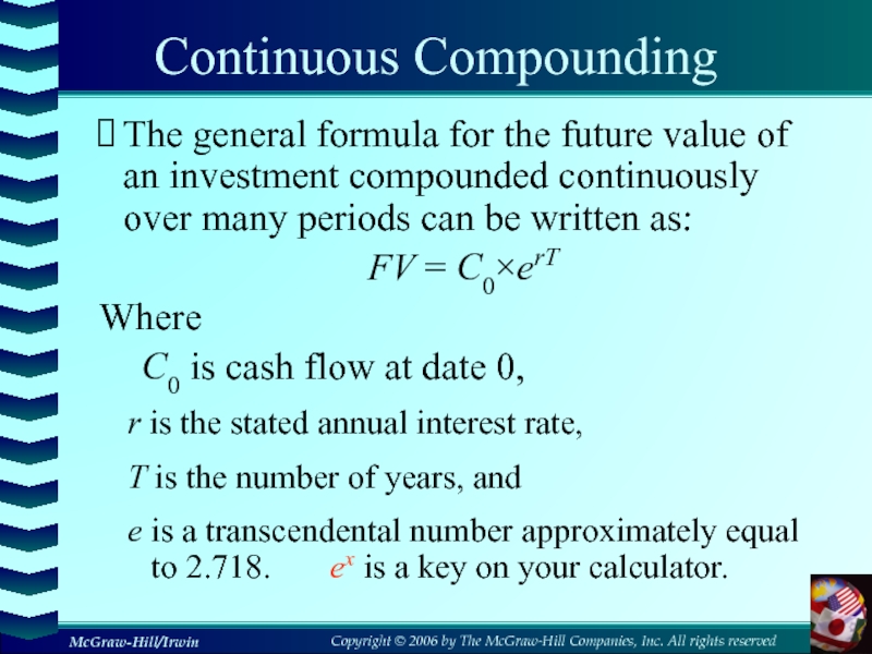
The general formula for the future value of an
investment compounded continuously over many periods can be written as:
FV
= C0×erTWhere
C0 is cash flow at date 0,
r is the stated annual interest rate,
T is the number of years, and
e is a transcendental number approximately equal to 2.718. ex is a key on your calculator.
Слайд 304.4 Simplifications
Annuity
A stream of constant cash flows that lasts for
a fixed number of periods
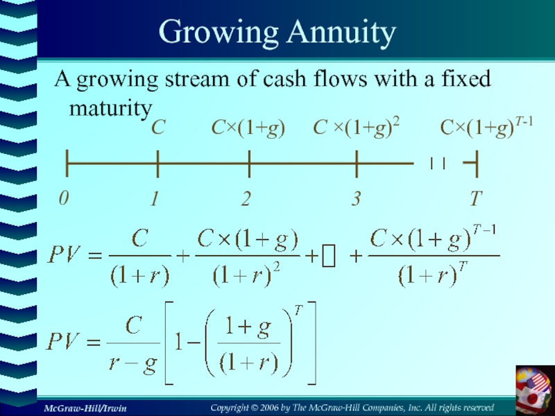
Growing annuity
A stream of cash flows
that grows at a constant rate for a fixed number of periodsPerpetuity
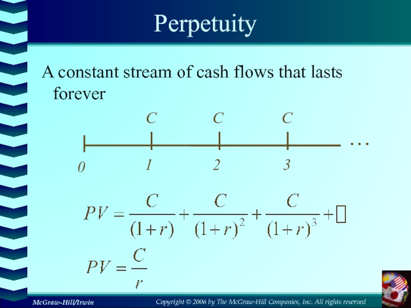
A constant stream of cash flows that lasts forever
Growing perpetuity
A stream of cash flows that grows at a constant rate forever
Слайд 32Annuity: Example
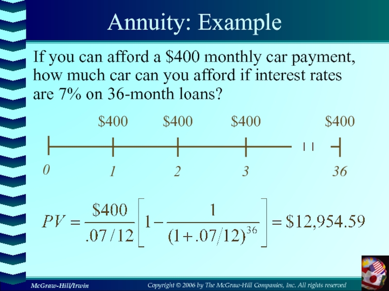
If you can afford a $400 monthly car payment,
how much car can you afford if interest rates are
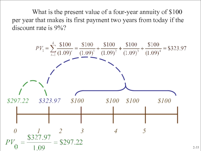
7% on 36-month loans?Слайд 33 What is the present value of a
four-year annuity of $100 per year that makes its first
payment two years from today if the discount rate is 9%?0 1 2 3 4 5
$100 $100 $100 $100
$323.97
$297.22
2-
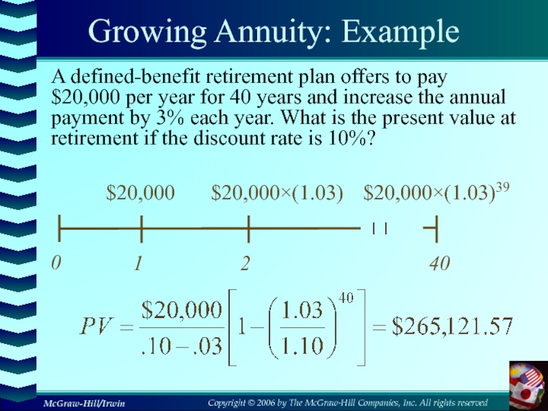
Слайд 35Growing Annuity: Example
A defined-benefit retirement plan offers to pay $20,000
per year for 40 years and increase the annual payment
by 3% each year. What is the present value at retirement if the discount rate is 10%?Слайд 37Perpetuity: Example
What is the value of a British consol that
promises to pay £15 every year for ever?
The interest
rate is 10-percent.…
Слайд 39Growing Perpetuity: Example
The expected dividend next year is $1.30, and
dividends are expected to grow at 5% forever.
If the
discount rate is 10%, what is the value of this promised dividend stream?…
Слайд 40Valuation of Bond and Stock
After reviewing the Time Value, then
we go to the main body of this chapter……
Слайд 419.1 Definition of a Bond
A bond is a legally binding
agreement between a borrower and a lender that specifies the:
Par
(face) valueCoupon rate
Coupon payment
Maturity Date
The yield to maturity is the required market interest rate on the bond.
Слайд 429.2 How to Value Bonds
Primary Principle:
Value of financial securities
= PV of expected future cash flows
Bond value is,
therefore, determined by the present value of the coupon payments and par value.Interest rates are inversely related to present (i.e., bond) values.
Слайд 44Pure Discount Bonds
Make no periodic interest payments (coupon rate =
0%)
The entire yield to maturity comes from the difference between
the purchase price and the par value.Cannot sell for more than par value
Sometimes called zeroes, deep discount bonds, or original issue discount bonds (OIDs)
Treasury Bills and principal-only Treasury strips are good examples of zeroes.
Слайд 45Pure Discount Bonds
Information needed for valuing pure discount bonds:
Time to
maturity (T) = Maturity date - today’s date
Face value (F)
Discount
rate (r)Present value of a pure discount bond at time 0:
Слайд 46Pure Discount Bond: Example
Find the value of a 30-year zero-coupon
bond with a $1,000 par value and a YTM of
6%.Слайд 47Level Coupon Bonds
Make periodic coupon payments in addition to the
maturity value
The payments are equal each period. Therefore, the bond
is just a combination of an annuity and a terminal (maturity) value.Coupon payments are typically semiannual.
Effective annual rate (EAR) =
(1 + R/m)m – 1
Слайд 48Level Coupon Bond: Example
Consider a U.S. government bond with a
6 3/8% coupon that expires in December 2010.
The Par Value
of the bond is $1,000.Coupon payments are made semi-annually (June 30 and December 31 for this particular bond).
Since the coupon rate is 6 3/8%, the payment is $31.875.
On January 1, 2006 the size and timing of cash flows are:
Слайд 50Bond Example: Calculator
PMT
I/Y
FV
PV
N
PV
31.875 =
2.5
1,000
– 1,060.17
10
Find the present value (as of
January 1, 2006), of a 6 3/8% coupon bond with
semi-annual payments, and a maturity date of December 2010 if the YTM is 5%.Слайд 51Bond Pricing with a Spreadsheet
There are specific formulas for finding
bond prices and yields on a spreadsheet.
PRICE(Settlement,Maturity,Rate,Yld,Redemption, Frequency,Basis)
YIELD(Settlement,Maturity,Rate,Pr,Redemption, Frequency,Basis)
Settlement and
maturity need to be actual datesThe redemption and Pr need to be given as % of par value
Click on the Excel icon for an example.
Слайд 52Consols
Not all bonds have a final maturity.
British consols pay a
set amount (i.e., coupon) every period forever.
These are examples of
a perpetuity.Слайд 539.3 Bond Concepts
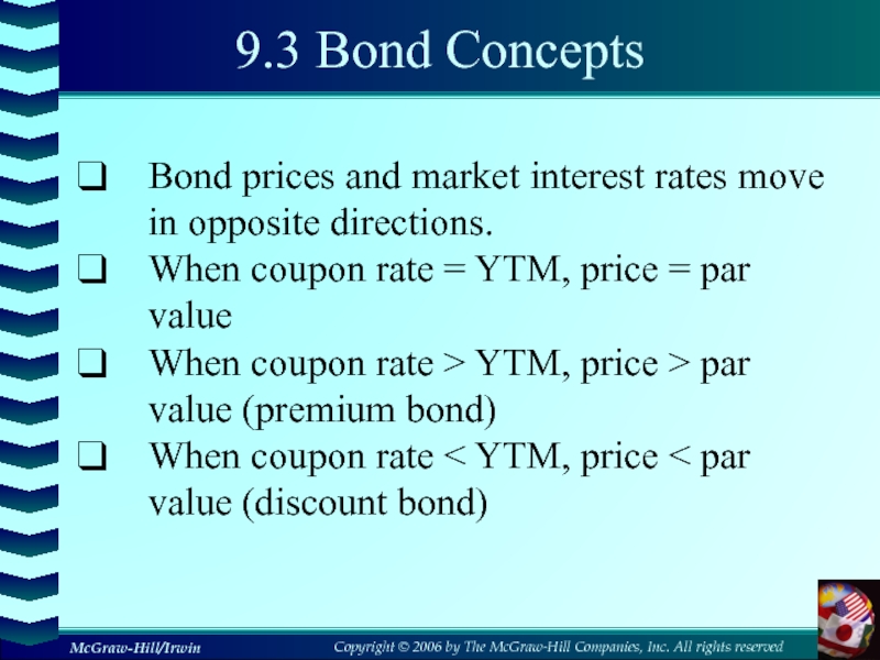
Bond prices and market interest rates move in
opposite directions.
When coupon rate = YTM, price = par value
When
coupon rate > YTM, price > par value (premium bond)When coupon rate < YTM, price < par value (discount bond)
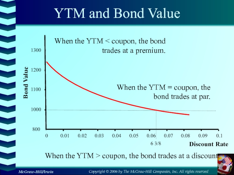
Слайд 54YTM and Bond Value
800
1000
1100
1200
1300
0
0.01
0.02
0.03
0.04
0.05
0.06
0.07
0.08
0.09
0.1
Discount Rate
Bond Value
When the YTM < coupon,
the bond trades at a premium.
When the YTM = coupon,
the bond trades at par.When the YTM > coupon, the bond trades at a discount.
Слайд 55Bond Example Revisited
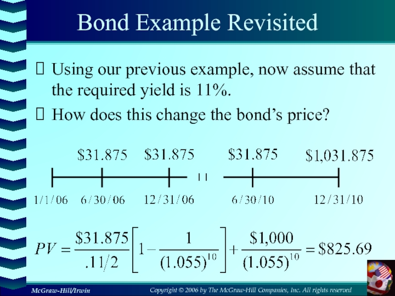
Using our previous example, now assume that the
required yield is 11%.
How does this change the bond’s
price?Слайд 56Computing Yield to Maturity
Yield to maturity is the rate implied
by the current bond price.
Finding the YTM requires trial and
error if you do not have a financial calculator and is similar to the process for finding R with an annuity.If you have a financial calculator, enter N, PV, PMT, and FV, remembering the sign convention (PMT and FV need to have the same sign, PV the opposite sign).
Слайд 57YTM with Annual Coupons
Consider a bond with a 10% annual
coupon rate, 15 years to maturity, and a par value
of $1,000. The current price is $928.09.Will the yield be more or less than 10%?
N = 15; PV = -928.09; FV = 1,000; PMT = 100
CPT I/Y = 11%
Слайд 58YTM with Semiannual Coupons
Suppose a bond with a 10% coupon
rate and semiannual coupons has a face value of $1,000,
20 years to maturity, and is selling for $1,197.93.Is the YTM more or less than 10%?
What is the semiannual coupon payment?
How many periods are there?
N = 40; PV = -1,197.93; PMT = 50; FV = 1,000; CPT I/Y = 4% (Is this the YTM?)
YTM = 4%*2 = 8%
Слайд 59Bond Market Reporting
Primarily over-the-counter transactions with dealers connected electronically
Extremely large
number of bond issues, but generally low daily volume in
single issuesMakes getting up-to-date prices difficult, particularly on a small company or municipal issues
Treasury securities are an exception
Слайд 60Treasury Quotations
8 Nov 21 132:23 132:24 -12 5.14
What is the coupon rate on
the bond?
When does the bond mature?
What is the bid price?
What does this mean?What is the ask price? What does this mean?
How much did the price change from the previous day?
What is the yield based on the ask price?
Слайд 61Slide
Range of values for equity
Earnings/cash flows under new ownership
Dividends
under existing ownership
Assets basis
Maximum value
Minimum value
Слайд 62Slide
Asset valuation bases
Possible bases of valuation
Historic
(unlikey to be realistic)
Replacement
(asset used on ongoing basis)
Realisable
(asset sold/ business broken up)
Слайд 63Assets basis
If a business is difficult to sell,
its owners may be prepared to accept a minimum bid
that matched the value that they get from a liquidation. There are 2 ways of assessing this:Balance sheet value - but the book value of assets will differ from their market value
Realisable value - better, but harder to calculate.
Slide
Слайд 649.4 The Present Value of Common Stocks
The value of any
asset is the present value of its expected future cash
flows.Stock ownership produces cash flows from:
Dividends
Capital Gains
Valuation of Different Types of Stocks
Zero Growth
Constant Growth
Differential Growth
Слайд 66Case 1: Zero Growth
Assume that dividends will remain at the
same level forever
Since future cash flows are constant, the value
of a zero growth stock is the present value of a perpetuity:Слайд 67Case 2: Constant Growth
Since future cash flows grow at a
constant rate forever, the value of a constant growth stock
is the present value of a growing perpetuity:Assume that dividends will grow at a constant rate, g, forever, i.e.,
.
.
.
Слайд 68Constant Growth Example
Suppose Big D, Inc., just paid a dividend
of $.50. It is expected to increase its dividend by
2% per year. If the market requires a return of 15% on assets of this risk level, how much should the stock be selling for?P0 = .50(1+.02) / (.15 - .02) = $3.92
Слайд 69Case 3: Differential Growth
Assume that dividends will grow at different
rates in the foreseeable future and then will grow at
a constant rate thereafter.To value a Differential Growth Stock, we need to:
Estimate future dividends in the foreseeable future.
Estimate the future stock price when the stock becomes a Constant Growth Stock (case 2).
Compute the total present value of the estimated future dividends and future stock price at the appropriate discount rate.
Слайд 70Case 3: Differential Growth
Assume that dividends will grow at rate
g1 for N years and grow at rate g2 thereafter.
.
.
.
.
.
.
Слайд 71Case 3: Differential Growth
Dividends will grow at rate g1 for
N years and grow at rate g2 thereafter
…
0
1 2 …
N N+1
…
Слайд 72Case 3: Differential Growth
We can value this as the sum
of:
an N-year annuity growing at rate g1
plus the discounted
value of a perpetuity growing at rate g2 that starts in year N+1Слайд 74A Differential Growth Example
A common stock just paid a dividend
of $2. The dividend is expected to grow at 8%
for 3 years, then it will grow at 4% in perpetuity.What is the stock worth? The discount rate is 12%.
Слайд 76With Cash Flows
…
0 1 2 3 4
0 1
2
3The constant growth phase beginning in year 4 can be valued as a growing perpetuity at time 3.
Слайд 77Disadvantages
Slide
It is difficult to estimating future dividend growth
It
is inaccurate to assume that growth will be constant
It
creates zero values for zero dividend companies. It creates negative values for high growth companies, if g > Ke
Слайд 78The Red Bud Co. just paid a dividend of $1.20
a share. The company announced today that it will continue
to pay this constant dividend for the next 3 years after which time it will discontinue paying dividends permanently. What is one share of this stock worth today if the required rate of return is 7%?a. $2.94
b. $3.15
c. $3.23
d. $3.44
e. $3.60
Слайд 799.5 Estimates of Parameters
The value of a firm depends upon
its growth rate, g, and its discount rate, R.
Where
does g come from?g = Retention ratio × Return on retained earnings
Слайд 80Where does R come from?
The discount rate can be broken
into two parts.
The dividend yield
The growth rate (in
dividends)In practice, there is a great deal of estimation error involved in estimating R.
Слайд 82what should be paid for Overland common stock? Overland has
just paid a dividend of $2.25. These dividends are expected
to grow at a rate of 5% in the foreseeable future. The required rate of return is 11%.Слайд 839.6 Growth Opportunities
Growth opportunities are opportunities to invest in positive NPV
projects.
The value of a firm can be conceptualized as the
sum of the value of a firm that pays out 100% of its earnings as dividends and the net present value of the growth opportunities.Слайд 849.7 The Dividend Growth Model and the NPVGO Model
We have
two ways to value a stock:
The dividend discount model
The sum
of its price as a “cash cow” plus the per share value of its growth opportunitiesСлайд 85The NPVGO Model: Example
Consider a firm that has
EPS of $5 at the end of the first year,
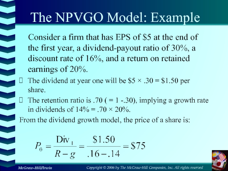
a dividend-payout ratio of 30%, a discount rate of 16%, and a return on retained earnings of 20%.The dividend at year one will be $5 × .30 = $1.50 per share.
The retention ratio is .70 ( = 1 -.30), implying a growth rate in dividends of 14% = .70 × 20%.
From the dividend growth model, the price of a share is:
Слайд 86The NPVGO Model: Example
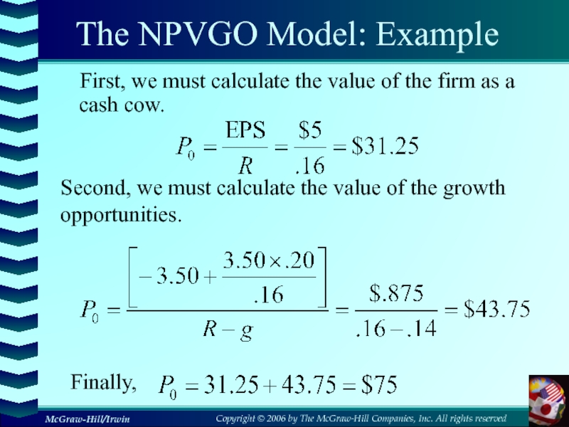
First, we must calculate the
value of the firm as a cash cow.
Second,
we must calculate the value of the growth opportunities. Finally,
Слайд 879.8 Price-Earnings Ratio
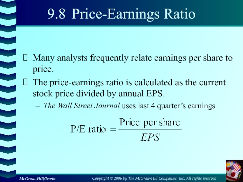
Many analysts frequently relate earnings per share to price.
The
price-earnings ratio is calculated as the current stock price divided
by annual EPS.The Wall Street Journal uses last 4 quarter’s earnings
Слайд 90Slide
Earnings basis - drawbacks
Market value = P/E
x Earnings
Which P/E?
Adjust downwards ?
One-off transactions?
Слайд 91Slide
Earnings yield
Market value = Earnings
Earnings yield
Earnings yield =
EPSMarket price per share
Слайд 92Valuation of other securities
Discounted cash flow techniques can be used
to value irredeemable debt, redeemable debt, convertible debt and preference
shares.Slide
Слайд 93Quick Quiz
How do you find the value of a bond,
and why do bond prices change?
What is a bond indenture,
and what are some of the important features?What determines the price of a share of stock?
What determines g and R in the DGM?
Decompose a stock’s price into constant growth and NPVGO values.
Discuss the importance of the PE ratio.
Слайд 94Lecture 9
Prospective Analysis – Valuation theory and concepts (part 2)
Chapter
7 – Palepu, Healy & Peek IFRS Edition
Слайд 95The steps involved in Business Analysis
Step 1 – Understanding the
Business
e.g.:
The Product market
The Competition
The Regulatory Constraints
Business strategies
Step 2 - Analyzing
Information – Accounting Analysis and Financial AnalysisQuality of Accounting information?
Re-formatting to uncover business activities
Ratio and cash flow analysis
Step 3 – Prospective analysis: Forecasting
Profit and Loss
Balance Sheet
Cash Flow
Step 4 – Prospective analysis: Valuation
RIM
Alternatives
Sensitivity
Step 5 – Application
for example:
Outside Investor
Compare Value with Price to BUY, SELL, or HOLD
Inside Investor
Compare Value with Cost to ACCEPT or REJECT Strategy
Strategy
22491 - Lecture 9 - Prospective Analysis - Valuation Part 2
Слайд 96Learning Objectives
At the conclusion of this lecture you should understand:
How to value a firm using the following methods:
Residual income
(Abnormal Earnings)Residual operating income
Discounted cash flow
22491 - Lecture 9 - Prospective Analysis - Valuation Part 2
Слайд 97Valuation
Is the process of converting the forecast into a valuation
of the assets of the business or the valuation of
shareholders’ equity.The different methods of business valuation include:
Dividend
Residual income model (Discounted Abnormal Earnings Method)
Residual Operating Income model
Free cash flow (DCF model)
Can use all to value either the equity or assets in the firm, (need to be sure which the model does!)
22491 - Lecture 9 - Prospective Analysis - Valuation Part 2
Слайд 98Earnings
Accountants and analysts focus on earnings
Earnings in the income statement
represent the flow of value “created” between two points in
time: NI1Distinguishable from dividends which are (net) flows paid back to the owners between two points in time: DIV1and dividends (and Book Value) – Relies on CSP (Clean Surplus Profit):
There is a relation between earnings BVE1 = BVE0 + CSP1 - DIV1
Or:
DIV1 = CSP1 + BVE0 - BVE1
CSP1 = BVE1 + DIV1 - BVE0
BVE0 = Book Value of Equity at START of Year
BVE1 = Book Value of Equity at END of Year
CSP1 = Clean Surplus Profit
DIV1 = Dividend Paid during year 1
22491 - Lecture 9 - Prospective Analysis - Valuation Part 2
Слайд 99Residual Income Model
Normal Earnings Capitalised
Abnormal Earnings (Residual Income) Capitalised
22491 -
Lecture 9 - Prospective Analysis - Valuation Part 2
Where re
is the cost of equity capitalСлайд 101Residual Income Model
Requires forecasts to infinity
Can forecast far enough into
the future that residual income approaches zero
Or need a finite
horizon forecast model22491 - Lecture 9 - Prospective Analysis - Valuation Part 2
Слайд 103Residual Income Model – Terminal Values
Choice of 3 simple ways
to calculate a terminal value at some time in the
future – our forecast horizon3 choices:
Residual Income = 0
Residual Income in perpetuity
Residual Income continues in perpetuity, with growth
Choice dependent on what we know of the firm, and therefore our forecasts
22491 - Lecture 9 - Prospective Analysis - Valuation Part 2
Слайд 104Residual Income Model– steps in valuation
Forecast CSP (Clean Surplus Profit)
and book values of equity
Estimate cost of capital for equity
Calculate
Residual Income = CSP – opening equity (for that year) x cost of capital for equityCalculate forecast Residual Income growth patterns to estimate Terminal Value (TV) calculation method (0, perpetuity or perpetuity with growth)
Calculate TV at time T (where growth pattern stabilises)
Discount forecast Residual Income to TV year and the TV, add together + opening book value for total value
22491 - Lecture 9 - Prospective Analysis - Valuation Part 2
Слайд 1051. Residual Income Model: AE = 0
Why would residual income
approach 0? = industry competition, government intervention
Remember:
22491 - Lecture 9
- Prospective Analysis - Valuation Part 2Слайд 1061. Residual Income Model: AE = 0
22491 - Lecture 9
- Prospective Analysis - Valuation Part 2
Слайд 1082. Residual Income Model:
AE continues in perpetuity
Most common finding
(mean reversion of returns)
22491 - Lecture 9 - Prospective Analysis
- Valuation Part 2Слайд 112Residual Income Model: practice question
Estimate the value of Charles’ company
using the abnormal earnings approach:
Слайд 113Residual Income Model:
practice question – Template solution
22491 - Lecture
9 - Prospective Analysis - Valuation Part 2
Слайд 114Residual Income Model:
practice question – Solution
22491 - Lecture 9
- Prospective Analysis - Valuation Part 2
Слайд 115Residual Income Model
Advantages:
Academic research shows that this method out performs
many of the other models
Focus on value drivers
Profitability of investment
and growth in investmentDirects strategic thinking
Incorporates the financial statements
Incorporates the balance sheet (book value)
Forecasts the income statement and the balance sheet
Uses accrual accounting
Recognizes value added
Matches value added to value lost
Treats investment as an asset
Versatility
Can be used with a wide variety of accounting principles
Aligned with what people forecast
Can be validated
Disadvantages:
Accounting Complexity
Requires understanding of how accounting works
Suspect accounting
Accounting numbers can be suspect
Forecast Horizon
Forecast horizon depends on the quality of the accounting
22491 - Lecture 9 - Prospective Analysis - Valuation Part 2
Слайд 116Residual Operating Income Model
(RIM Modified)
Residual Income Model– uses cost
of capital (equity)
Cost of capital (equity) = changes every time
leverage changes (cost of capital debt)Residual Operating Income Model – uses cost of capital (firm)
Value of equity = value of assets (firm) – value of debt
22491 - Lecture 9 - Prospective Analysis - Valuation Part 2
Слайд 117Residual Operating Income Model
Therefore - can also estimate equity values
by calculating the value of assets and subtracting the book
value of debt (often simpler – no need to think about leverage)Value of Equity = Value of Assets – Book Value of Debt
Question: So how to value the assets (firm)?
Equity = NOA – Net debt (NFL)
CSP = NOPAT – Net financing expenses
NOA = Net Operating Assets
CSP = Clean Surplus Profit
Net Debt = Net Financial Liabilities = Interest Bearing Debt (Current + Non Current) – (Cash +Cash Equivalents)
NOPAT = Net Operating Profit after tax
Net Financing Expense = Interest Expense – Interest Revenue
22491 - Lecture 9 - Prospective Analysis - Valuation Part 2
Слайд 118Residual OPERATING Income Model
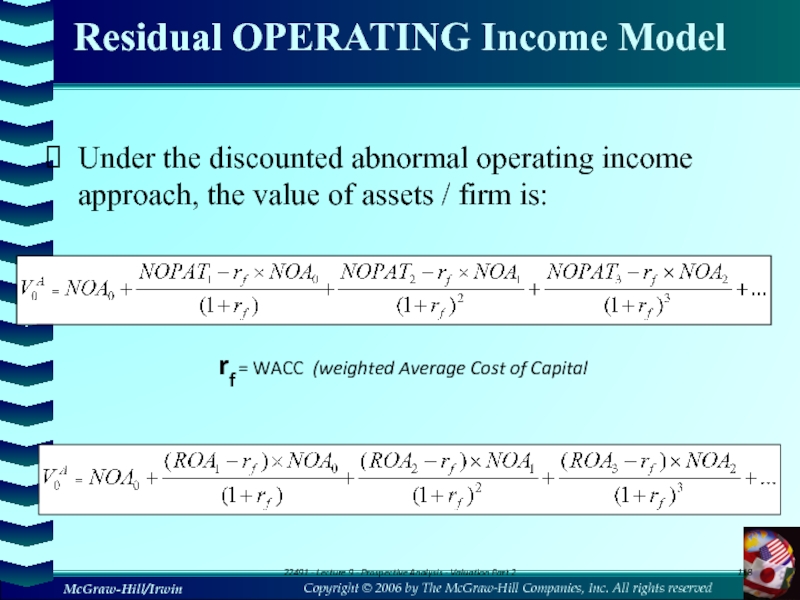
Under the discounted abnormal operating income approach,
the value of assets / firm is:
22491 - Lecture 9
- Prospective Analysis - Valuation Part 2rf = WACC (weighted Average Cost of Capital
Слайд 119Residual Operating Income Model
Gives the same result as abnormal earnings
valuation (as long as cost of capital for equity is
adjusted each time leverage changes)22491 - Lecture 9 - Prospective Analysis - Valuation Part 2
Слайд 120Residual Operating Income Model - steps
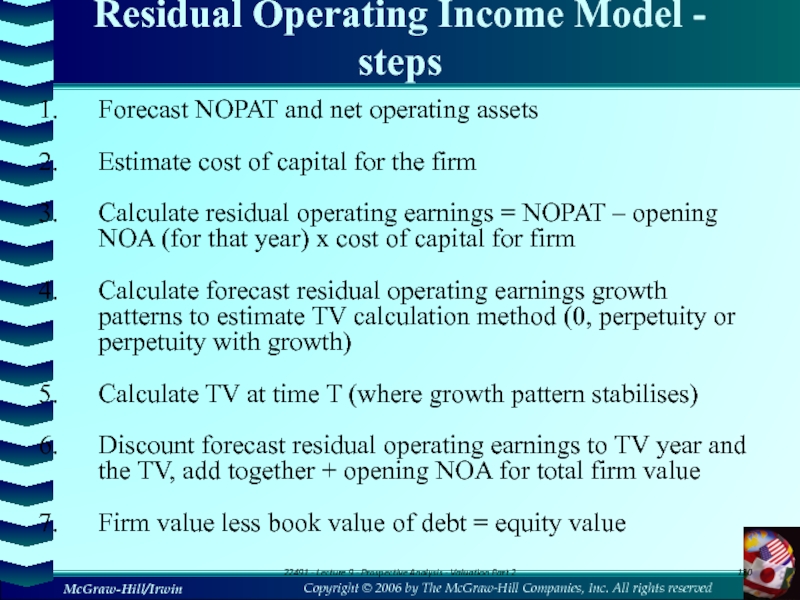
Forecast NOPAT and net operating
assets
Estimate cost of capital for the firm
Calculate residual operating earnings
= NOPAT – opening NOA (for that year) x cost of capital for firmCalculate forecast residual operating earnings growth patterns to estimate TV calculation method (0, perpetuity or perpetuity with growth)
Calculate TV at time T (where growth pattern stabilises)
Discount forecast residual operating earnings to TV year and the TV, add together + opening NOA for total firm value
Firm value less book value of debt = equity value
22491 - Lecture 9 - Prospective Analysis - Valuation Part 2
Слайд 121Residual Operating Income Model - question
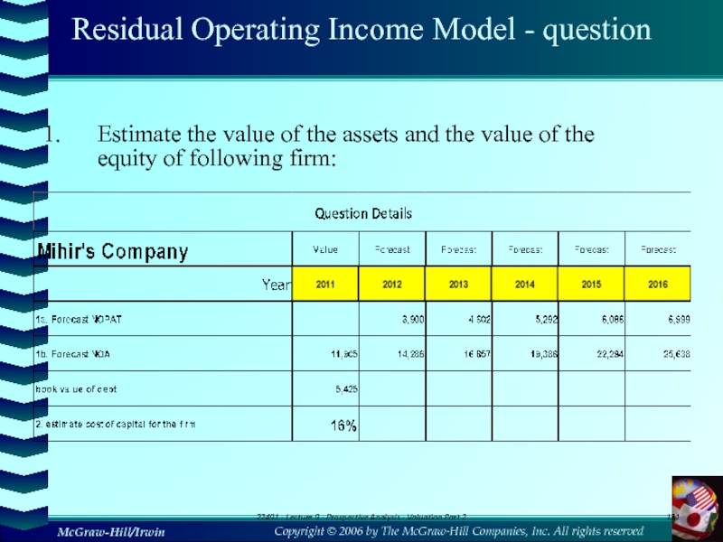
Estimate the value of the
assets and the value of the equity of following firm:
22491
- Lecture 9 - Prospective Analysis - Valuation Part 2Слайд 122Residual OPERATING Income Model – Solution Template
22491 - Lecture 9
- Prospective Analysis - Valuation Part 2
Слайд 123Residual OPERATING Income Model - solution
22491 - Lecture 9 -
Prospective Analysis - Valuation Part 2
Слайд 124Free Cash Flow (DCF) Model
Similar to the residual operating income
model
Accounting without accruals
Free Cash Flows (FCF) = NOPAT - ∆Net
Operating AssetsNOA = 0
rf = WACC
22491 - Lecture 9 - Prospective Analysis - Valuation Part 2
Слайд 125Also forecasts over an infinite horizon: need to make a
terminal assumption:
No FCF past horizon
Capitalise terminal free cash flow as
a perpetuity, orCapitalise terminal free cash flow as a perpetuity with growth
The Continuing Value for the DCF
22491 - Lecture 9 - Prospective Analysis - Valuation Part 2
Слайд 126DCF valuation method - steps
Forecast free cash flow
Estimate cost of
capital for the firm
Calculate forecast FCF growth patterns to estimate
Terminal Value (TV) calculation method (0, perpetuity or perpetuity with growth)Calculate TV at time T (where growth pattern stabilises)
Discount forecast FCF to TV year and the TV, add together for total firm value
Firm value less Book Value of DEBT = Equity Value
22491 - Lecture 9 - Prospective Analysis - Valuation Part 2
Слайд 130What are the problems with DCF?
Cash flow from operations (value
added) is reduced by investments (which also add value): investments
are treated as value lossesValue received is not matched against value surrendered to generate value - except for long forecast horizons
Note: analysts forecast earnings, not cash flows
22491 - Lecture 9 - Prospective Analysis - Valuation Part 2
Слайд 131DCF Analysis
Advantages
Easy concept: cash flows are “real” and easy to think
about; they are not
affected by accounting rules
Familiarity:
is a straight application of familiar net present valuetechniques
Disadvantages
Suspect concept: → free cash flow does not measure value added in the
short run; value gained is not matched with value given up
→ free cash flow fails to recognize value generated that
does not involve cash flows
→ investment is treated as a loss of value
→ free cash flow is partly a liquidation concept; firms
increase free cash flow by cutting back on investments
Forecast horizons: can require long forecast horizons to recognize cash
inflows from investments, particularly when investments
are growing
Validation: it is hard to validate free cash flow forecasts
Not aligned with
what people
forecast: analysts forecast earnings, not free cash flow; adjusting
earnings forecasts to free cash forecasts requires further
forecasting of accruals
When It Works Best
When the investment pattern is such as to produce constant free cash flow or free cash flow growing at a constant rate
22491 - Lecture 9 - Prospective Analysis - Valuation Part 2
Слайд 132Comparing the models – DDM, DCF and RIM
All derive from
the dividend discount model
Differences:
Focus on different issues
Require different levels of
structureHave different implications for terminal values
22491 - Lecture 9 - Prospective Analysis - Valuation Part 2
Слайд 133Comparing the models – DDM, DCF and RIM(DAE) – research
results
Penman and Suogiannis (1998) CAR
Dechow Hutton and Sloan (1999) JAE
Francis,
Olsson and Oswald (2000) JAROver relatively short forecast horizons (ten years or less) valuation estimates using DAE are more precise than DDM or DCF
Advantage persists over both conservative and aggressive accounting = US results that accrual accounting reflects future cash flows
22491 - Lecture 9 - Prospective Analysis - Valuation Part 2
Слайд 134Summary
Valuation converts forecasts of performance into approximated market price
There are
3 methods derived from DDM, namely
Residual Income model, Residual
Operating Income model and the DCF model (using Free Cash Flows) each has advantages and disadvantages so there are gains in considering using all of the approachesPrice multiples can also be used. These have been popular as there is no need for multi year forecasts. However, finding benchmark firms is difficult
22491 - Lecture 9 - Prospective Analysis - Valuation Part 2
