Разделы презентаций
- Разное
- Английский язык
- Астрономия
- Алгебра
- Биология
- География
- Геометрия
- Детские презентации
- Информатика
- История
- Литература
- Математика
- Медицина
- Менеджмент
- Музыка
- МХК
- Немецкий язык
- ОБЖ
- Обществознание
- Окружающий мир
- Педагогика
- Русский язык
- Технология
- Физика
- Философия
- Химия
- Шаблоны, картинки для презентаций
- Экология
- Экономика
- Юриспруденция
Chap 3- 1 Copyright ©2013 Pearson Education, Inc. publishing as Prentice
Содержание
- 1. Chap 3- 1 Copyright ©2013 Pearson Education, Inc. publishing as Prentice
- 2. Chap 3-Copyright ©2013 Pearson Education, Inc. publishing
- 3. Chap 3-Copyright ©2013 Pearson Education, Inc. publishing
- 4. Chap 3-Copyright ©2013 Pearson Education, Inc. publishing
- 5. Chap 3-Copyright ©2013 Pearson Education, Inc. publishing
- 6. Chap 3-Copyright ©2013 Pearson Education, Inc. publishing
- 7. Chap 3-Copyright ©2013 Pearson Education, Inc. publishing
- 8. Chap 3-Copyright ©2013 Pearson Education, Inc. publishing
- 9. Chap 3-Copyright ©2013 Pearson Education, Inc. publishing
- 10. Chap 3-Copyright ©2013 Pearson Education, Inc. publishing
- 11. Chap 3-Copyright ©2013 Pearson Education, Inc. publishing
- 12. Chap 3-Copyright ©2013 Pearson Education, Inc. publishing
- 13. Chap 3-Copyright ©2013 Pearson Education, Inc. publishing
- 14. Chap 3-Copyright ©2013 Pearson Education, Inc. publishing
- 15. Chap 3-Copyright ©2013 Pearson Education, Inc. publishing
- 16. Chap 3-Copyright ©2013 Pearson Education, Inc. publishing
- 17. Chap 3-Copyright ©2013 Pearson Education, Inc. publishing
- 18. Chap 3-Copyright ©2013 Pearson Education, Inc. publishing
- 19. Chap 3-Copyright ©2013 Pearson Education, Inc. publishing
- 20. Chap 3-Copyright ©2013 Pearson Education, Inc. publishing
- 21. Chap 3-
- 22. Chap 3-Copyright ©2013 Pearson Education, Inc. publishing
- 23. Chap 3-Copyright ©2013 Pearson Education, Inc. publishing
- 24. Chap 3-Copyright ©2013 Pearson Education, Inc. publishing
- 25. Chap 3-Copyright ©2013 Pearson Education, Inc. publishing
- 26. Chap 3-Copyright ©2013 Pearson Education, Inc. publishing
- 27. Chap 3-Copyright ©2013 Pearson Education, Inc. publishing
- 28. Chap 3-Copyright ©2013 Pearson Education, Inc. publishing
- 29. Chap 3-Copyright ©2013 Pearson Education, Inc. publishing
- 30. Chap 3-Copyright ©2013 Pearson Education, Inc. publishing
- 31. Chap 3-Copyright ©2013 Pearson Education, Inc. publishing
- 32. Shape of a Distribution -- Kurtosis measures
- 33. Chap 3-Copyright ©2013 Pearson Education, Inc. publishing
- 34. Chap 3-Copyright ©2013 Pearson Education, Inc. publishing
- 35. Chap 3-Copyright ©2013 Pearson Education, Inc. publishing
- 36. Chap 3-Copyright ©2013 Pearson Education, Inc. publishing
- 37. Chap 3-Copyright ©2013 Pearson Education, Inc. publishing
- 38. Chap 3-Copyright ©2013 Pearson Education, Inc. publishing
- 39. Chap 3-Copyright ©2013 Pearson Education, Inc. publishing
- 40. Chap 3-Copyright ©2013 Pearson Education, Inc. publishing
- 41. Chap 3-Copyright ©2013 Pearson Education, Inc. publishing
- 42. Chap 3-Copyright ©2013 Pearson Education, Inc. publishing
- 43. Chap 3-Copyright ©2013 Pearson Education, Inc. publishing
- 44. Chap 3-Copyright ©2013 Pearson Education, Inc. publishing
- 45. Chap 3-Copyright ©2013 Pearson Education, Inc. publishing
- 46. Chap 3-Copyright ©2013 Pearson Education, Inc. publishing
- 47. Chap 3-Copyright ©2013 Pearson Education, Inc. publishing
- 48. Chap 3-Copyright ©2013 Pearson Education, Inc. publishing
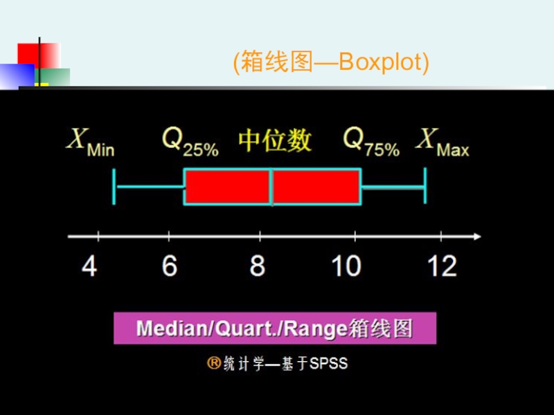
- 49. (箱线图—Boxplot)
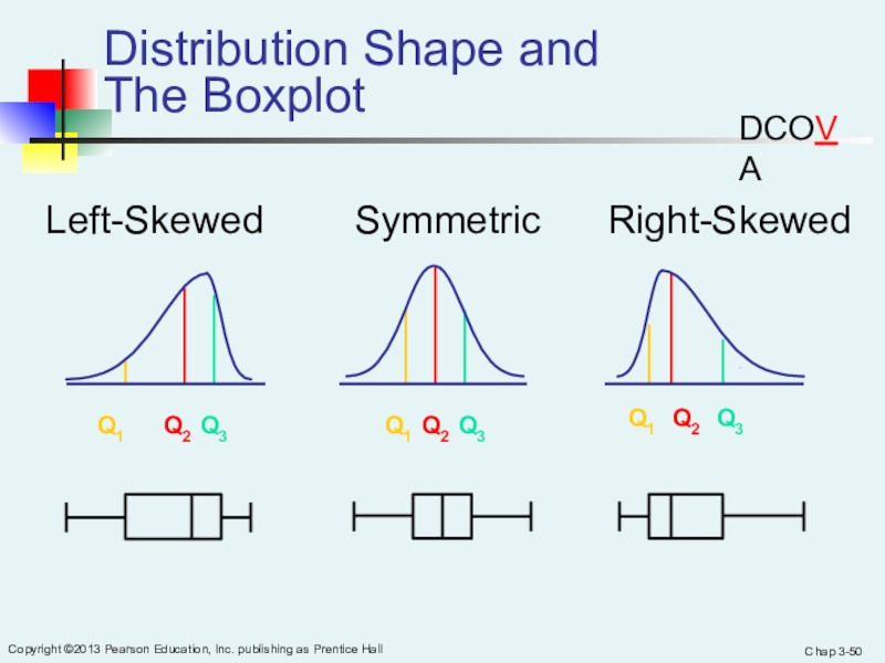
- 50. Chap 3-Copyright ©2013 Pearson Education, Inc. publishing as Prentice Hall Distribution Shape and The BoxplotRight-SkewedLeft-SkewedSymmetricQ1Q2Q3Q1Q2Q3Q1Q2Q3DCOVA
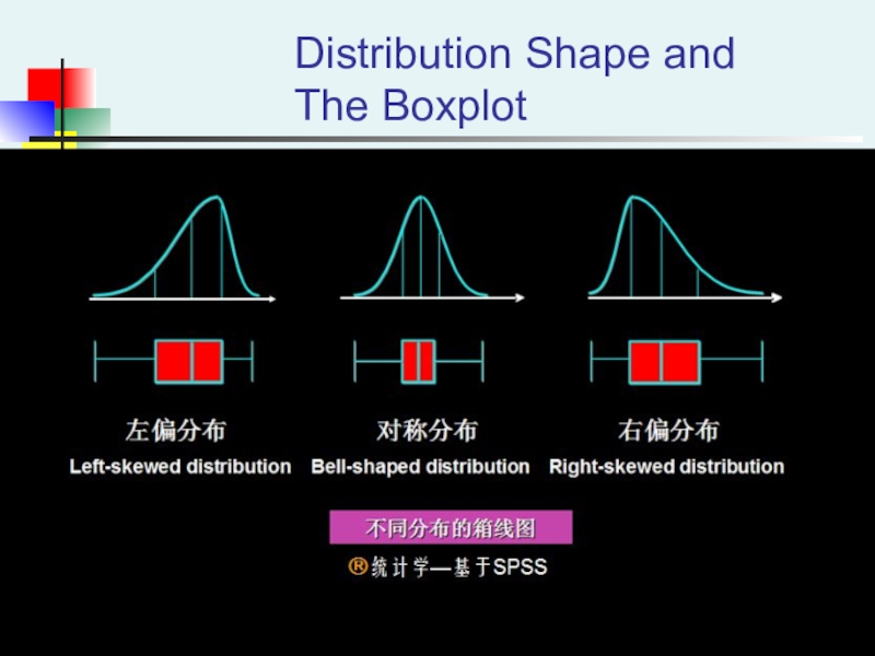
- 51. Distribution Shape and The Boxplot
- 52. Chap 3-Copyright ©2013 Pearson Education, Inc. publishing
- 53. Chap 3-Copyright ©2013 Pearson Education, Inc. publishing
- 54. Chap 3-Copyright ©2013 Pearson Education, Inc. publishing
- 55. Chap 3-Copyright ©2013 Pearson Education, Inc. publishing
- 56. Chap 3-Copyright ©2013 Pearson Education, Inc. publishing
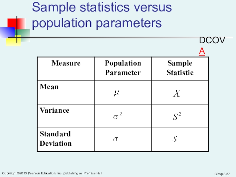
- 57. Chap 3-Copyright ©2013 Pearson Education, Inc. publishing as Prentice Hall Sample statistics versus population parametersDCOVA
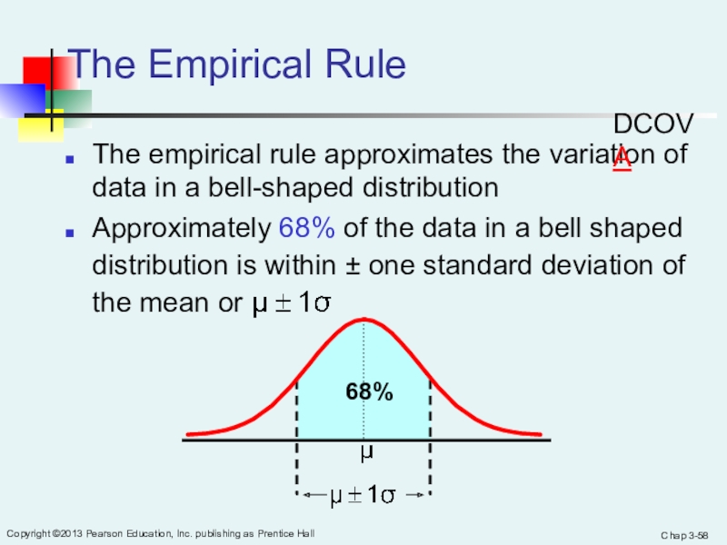
- 58. Chap 3-Copyright ©2013 Pearson Education, Inc. publishing
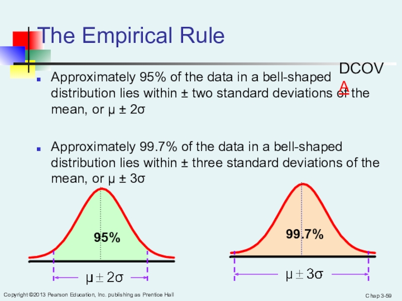
- 59. Chap 3-Copyright ©2013 Pearson Education, Inc. publishing
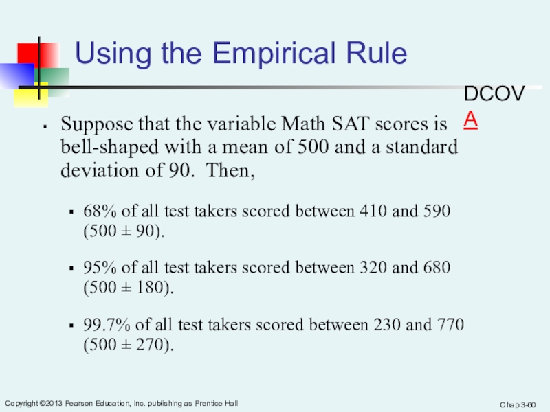
- 60. Chap 3-Copyright ©2013 Pearson Education, Inc. publishing
- 61. Chap 3-Copyright ©2013 Pearson Education, Inc. publishing
- 62. Chap 3-Copyright ©2013 Pearson Education, Inc. publishing
- 63. Chap 3-Copyright ©2013 Pearson Education, Inc. publishing
- 64. Chap 3-Copyright ©2013 Pearson Education, Inc. publishing
- 65. Chap 3-Copyright ©2013 Pearson Education, Inc. publishing
- 66. Chap 3-Copyright ©2013 Pearson Education, Inc. publishing
- 67. Chap 3-Copyright ©2013 Pearson Education, Inc. publishing
- 68. Chap 3-Copyright ©2013 Pearson Education, Inc. publishing
- 69. Chap 3-Copyright ©2013 Pearson Education, Inc. publishing
- 70. Chap 3-Copyright ©2013 Pearson Education, Inc. publishing
- 71. Chap 3-Copyright ©2013 Pearson Education, Inc. publishing as Prentice Hall The Coefficient of Correlation Using Minitab
- 72. Chap 3-Copyright ©2013 Pearson Education, Inc. publishing
- 73. Chap 3-Copyright ©2013 Pearson Education, Inc. publishing
- 74. Chap 3-Copyright ©2013 Pearson Education, Inc. publishing
- 75. Chap 3-Copyright ©2013 Pearson Education, Inc. publishing
- 76. Slide 3- Copyright © 2011 Pearson Education,
- 77. Slide 5- Copyright © 2011 Pearson Education,
- 78. Based on the histogram, what can we
- 79. Slide 5- Copyright © 2011 Pearson Education,
- 80. Slide 5- Copyright © 2011 Pearson Education,
- 81. Slide 5- Copyright © 2011 Pearson Education,
- 82. Slide 5- Copyright © 2011 Pearson Education,
- 83. Slide 5- Copyright © 2011 Pearson Education,
- 84. Slide 5- Copyright © 2011 Pearson Education,
- 85. Slide 5- Copyright © 2011 Pearson Education,
- 86. Slide 5- Copyright © 2011 Pearson Education,
- 87. Скачать презентанцию
Слайды и текст этой презентации
Слайд 2Chap 3-
Copyright ©2013 Pearson Education, Inc. publishing as Prentice Hall
In this chapter, you learn:
To describe the properties of
central tendency, variation, and shape in numerical dataTo construct and interpret a boxplot
To compute descriptive summary measures for a population
To compute the covariance and the coefficient of correlation
Learning Objectives
Слайд 3Chap 3-
Copyright ©2013 Pearson Education, Inc. publishing as Prentice Hall
Summary Definitions
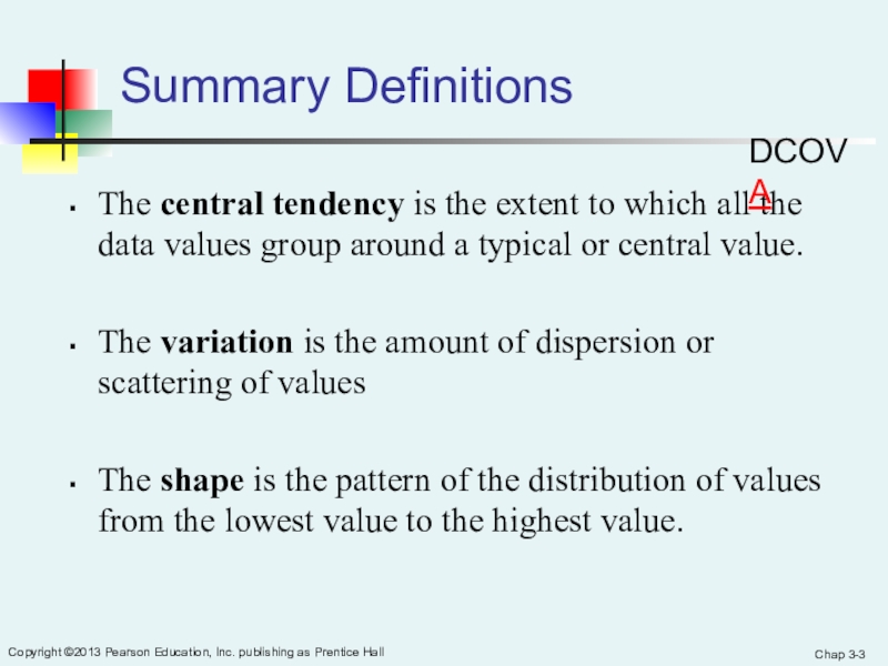
The central tendency is the extent to which all
the data values group around a typical or central value.The variation is the amount of dispersion or scattering of values
The shape is the pattern of the distribution of values from the lowest value to the highest value.
DCOVA
Слайд 4Chap 3-
Copyright ©2013 Pearson Education, Inc. publishing as Prentice Hall
Measures of Central Tendency:
The Mean
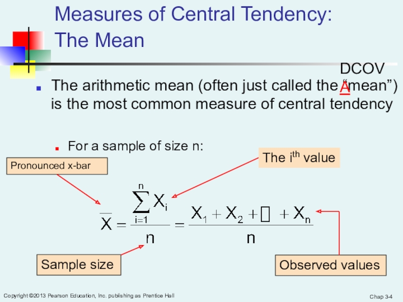
The arithmetic mean (often just called
the “mean”) is the most common measure of central tendencyFor a sample of size n:
Sample size
Observed values
The ith value
Pronounced x-bar
DCOVA
Слайд 5Chap 3-
Copyright ©2013 Pearson Education, Inc. publishing as Prentice Hall
Measures of Central Tendency:
The Mean
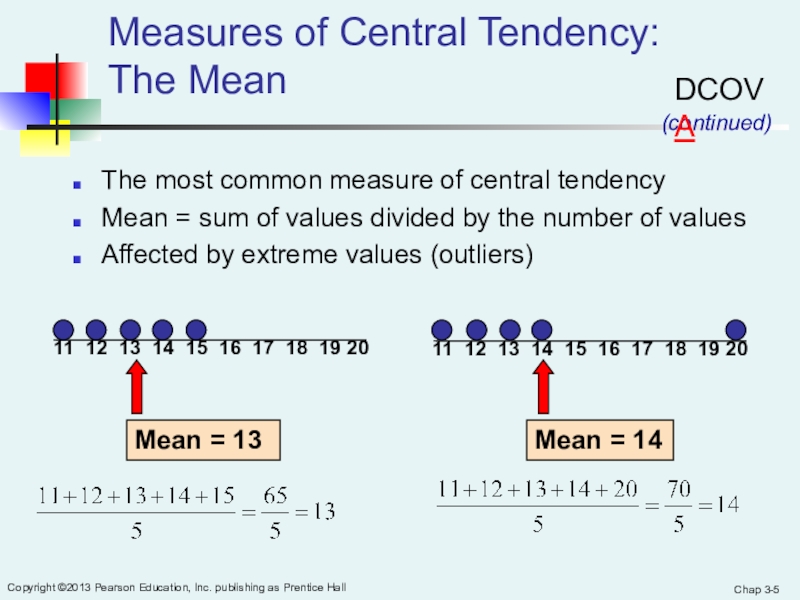
The most common measure of central
tendencyMean = sum of values divided by the number of values
Affected by extreme values (outliers)
(continued)
11 12 13 14 15 16 17 18 19 20
Mean = 13
11 12 13 14 15 16 17 18 19 20
Mean = 14
DCOVA
Слайд 6Chap 3-
Copyright ©2013 Pearson Education, Inc. publishing as Prentice Hall
Measures of Central Tendency:
The Median
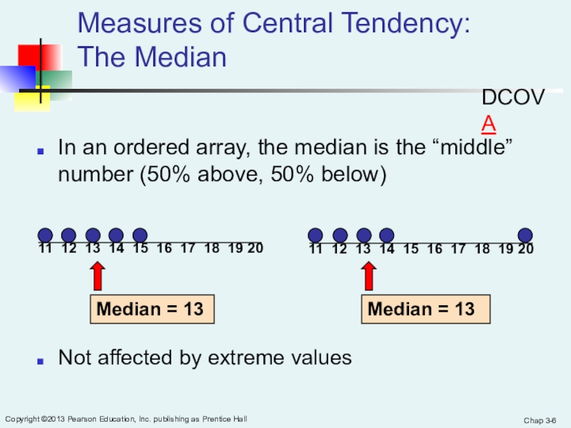
In an ordered array, the median
is the “middle” number (50% above, 50% below)Not affected by extreme values
Median = 13
Median = 13
11 12 13 14 15 16 17 18 19 20
11 12 13 14 15 16 17 18 19 20
DCOVA
Слайд 7Chap 3-
Copyright ©2013 Pearson Education, Inc. publishing as Prentice Hall
Measures of Central Tendency:
Locating the Median
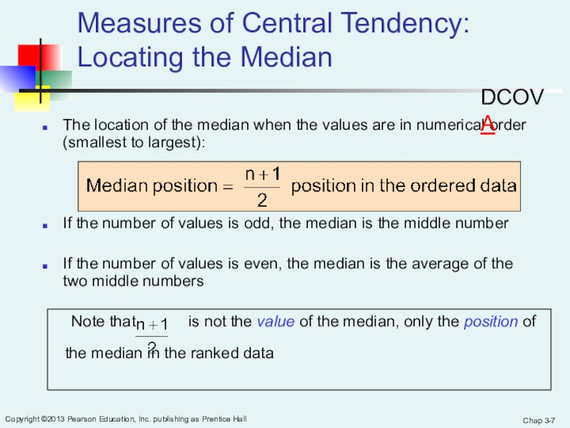
The location of the median
when the values are in numerical order (smallest to largest):If the number of values is odd, the median is the middle number
If the number of values is even, the median is the average of the two middle numbers
Note that is not the value of the median, only the position of
the median in the ranked data
DCOVA
Слайд 8Chap 3-
Copyright ©2013 Pearson Education, Inc. publishing as Prentice Hall
Measures of Central Tendency:
The Mode
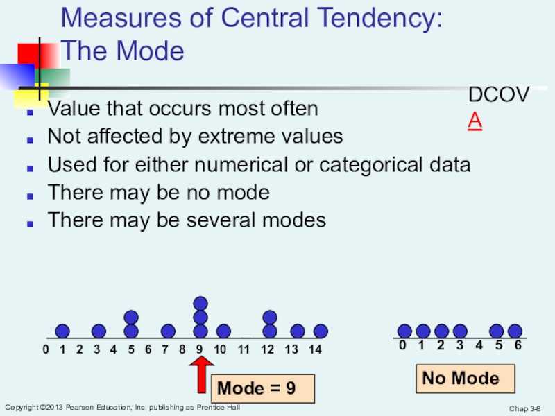
Value that occurs most often
Not affected
by extreme valuesUsed for either numerical or categorical data
There may be no mode
There may be several modes
0 1 2 3 4 5 6 7 8 9 10 11 12 13 14
Mode = 9
0 1 2 3 4 5 6
No Mode
DCOVA
Слайд 9Chap 3-
Copyright ©2013 Pearson Education, Inc. publishing as Prentice Hall
Measures of Central Tendency:
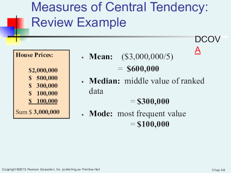
Review Example
House Prices:
$2,000,000$ 500,000 $ 300,000 $ 100,000 $ 100,000
Sum $ 3,000,000
Mean: ($3,000,000/5)
= $600,000
Median: middle value of ranked data
= $300,000
Mode: most frequent value
= $100,000
DCOVA
Слайд 10Chap 3-
Copyright ©2013 Pearson Education, Inc. publishing as Prentice Hall
Measures of Central Tendency:
Which Measure to Choose?
The mean is generally
used, unless extreme values (outliers) exist.The median is often used, since the median is not sensitive to extreme values. For example, median home prices may be reported for a region; it is less sensitive to outliers.
In some situations it makes sense to report both the mean and the median.
DCOVA
Слайд 11Chap 3-
Copyright ©2013 Pearson Education, Inc. publishing as Prentice Hall
Measures of Central Tendency:
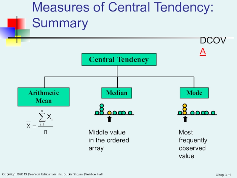
Summary
Central Tendency
Arithmetic Mean
Median
Mode
Middle value in the ordered
arrayMost frequently observed value
DCOVA
Слайд 12Chap 3-
Copyright ©2013 Pearson Education, Inc. publishing as Prentice Hall
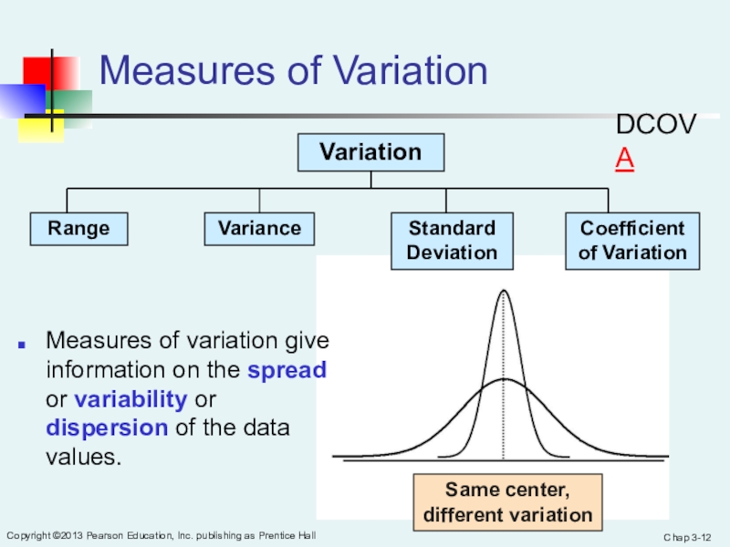
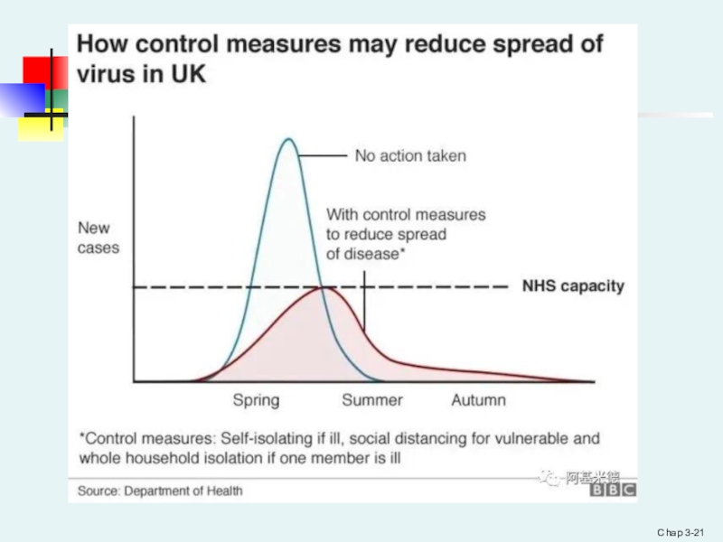
Same center,
different variation
Measures of Variation
Measures of variation give information
on the spread or variability or dispersion of the data values.
DCOVA
Слайд 13Chap 3-
Copyright ©2013 Pearson Education, Inc. publishing as Prentice Hall
Measures of Variation:
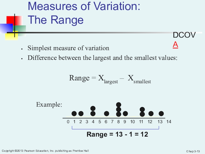
The Range
Simplest measure of variation
Difference between the largest
and the smallest values:Range = Xlargest – Xsmallest
0 1 2 3 4 5 6 7 8 9 10 11 12 13 14
Range = 13 - 1 = 12
Example:
DCOVA
Слайд 14Chap 3-
Copyright ©2013 Pearson Education, Inc. publishing as Prentice Hall
Measures of Variation:
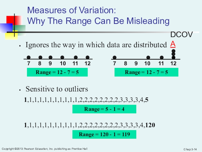
Why The Range Can Be Misleading
Ignores the way
in which data are distributedSensitive to outliers
7 8 9 10 11 12
Range = 12 - 7 = 5
7 8 9 10 11 12
Range = 12 - 7 = 5
1,1,1,1,1,1,1,1,1,1,1,2,2,2,2,2,2,2,2,3,3,3,3,4,5
1,1,1,1,1,1,1,1,1,1,1,2,2,2,2,2,2,2,2,3,3,3,3,4,120
Range = 5 - 1 = 4
Range = 120 - 1 = 119
DCOVA
Слайд 15Chap 3-
Copyright ©2013 Pearson Education, Inc. publishing as Prentice Hall
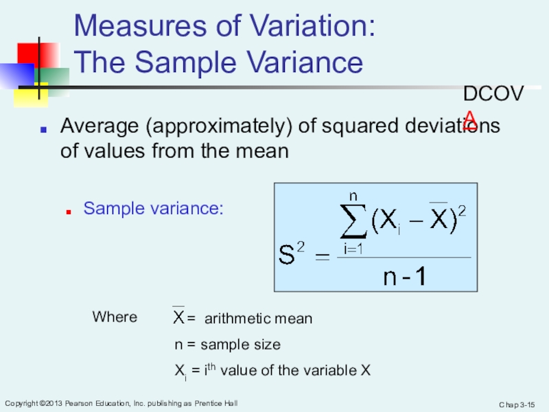
Average (approximately) of squared deviations of values from the mean
Sample
variance:Measures of Variation:
The Sample Variance
Where
= arithmetic mean
n = sample size
Xi = ith value of the variable X
DCOVA
Слайд 16Chap 3-
Copyright ©2013 Pearson Education, Inc. publishing as Prentice Hall
Measures of Variation:
The Sample Standard Deviation
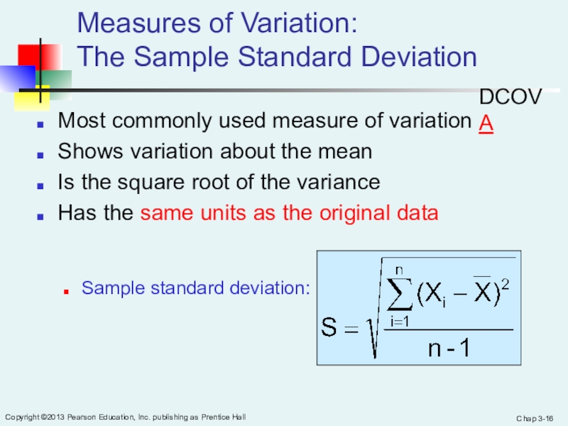
Most commonly used measure of
variationShows variation about the mean
Is the square root of the variance
Has the same units as the original data
Sample standard deviation:
DCOVA
Слайд 17Chap 3-
Copyright ©2013 Pearson Education, Inc. publishing as Prentice Hall
Measures of Variation:
The Standard Deviation
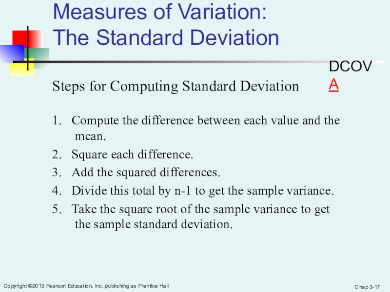
Steps for Computing Standard Deviation
1. Compute the
difference between each value and the mean.2. Square each difference.
3. Add the squared differences.
4. Divide this total by n-1 to get the sample variance.
5. Take the square root of the sample variance to get the sample standard deviation.
DCOVA
Слайд 18Chap 3-
Copyright ©2013 Pearson Education, Inc. publishing as Prentice Hall
Measures of Variation:
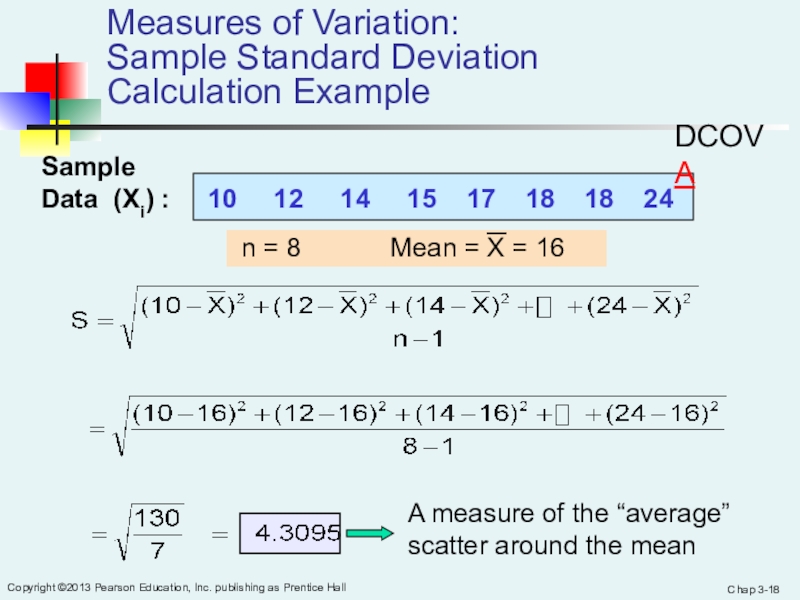
Sample Standard Deviation
Calculation Example
Sample
Data (Xi) :
10 12 14 15 17 18 18 24 n = 8 Mean = X = 16
A measure of the “average” scatter around the mean
DCOVA
Слайд 19Chap 3-
Copyright ©2013 Pearson Education, Inc. publishing as Prentice Hall
Measures of Variation:
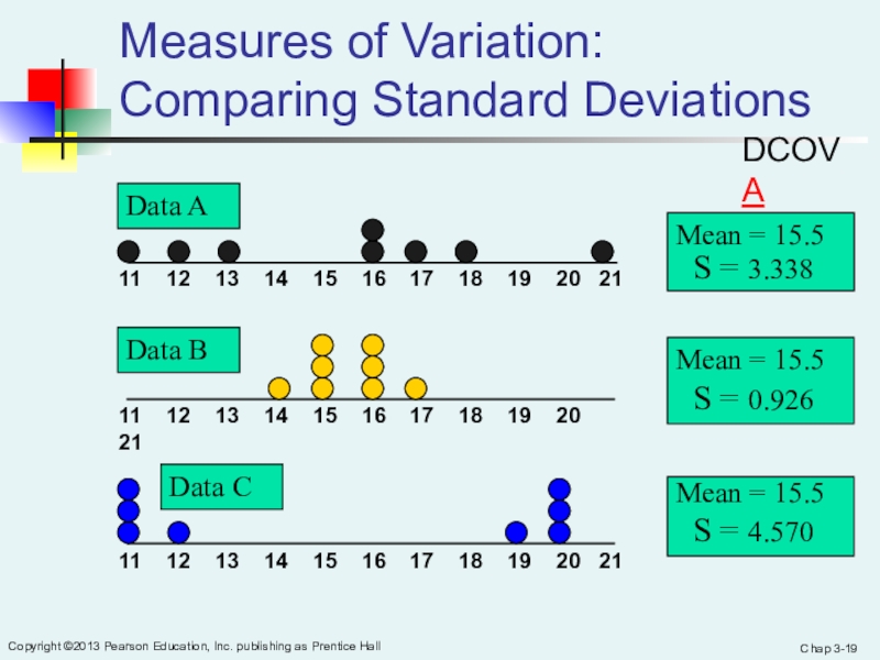
Comparing Standard Deviations
Mean = 15.5
S = 3.338
11 12 13 14 15 16 17 18 19 20 21
11 12 13 14 15 16 17 18 19 20 21
Data B
Data A
Mean = 15.5
S = 0.926
11 12 13 14 15 16 17 18 19 20 21
Mean = 15.5
S = 4.570
Data C
DCOVA
Слайд 20Chap 3-
Copyright ©2013 Pearson Education, Inc. publishing as Prentice Hall
Measures of Variation:
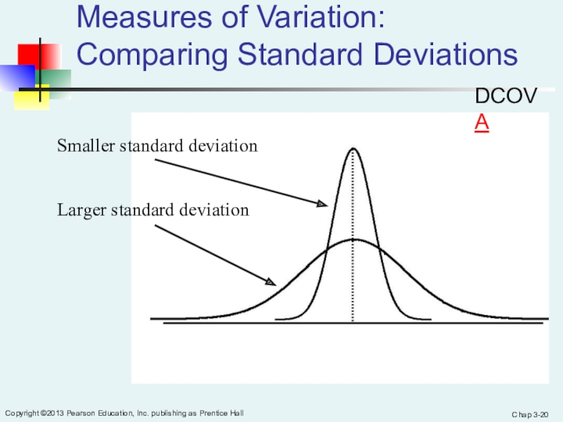
Comparing Standard Deviations
Smaller standard deviation
Larger standard deviation
DCOVA
Слайд 22Chap 3-
Copyright ©2013 Pearson Education, Inc. publishing as Prentice Hall
Measures of Variation:
Summary Characteristics
The more the data are spread out,
the greater the range, variance, and standard deviation.The more the data are concentrated, the smaller the range, variance, and standard deviation.
If the values are all the same (no variation), all these measures will be zero.
None of these measures are ever negative.
DCOVA
Слайд 23Chap 3-
Copyright ©2013 Pearson Education, Inc. publishing as Prentice Hall
Measures of Variation:
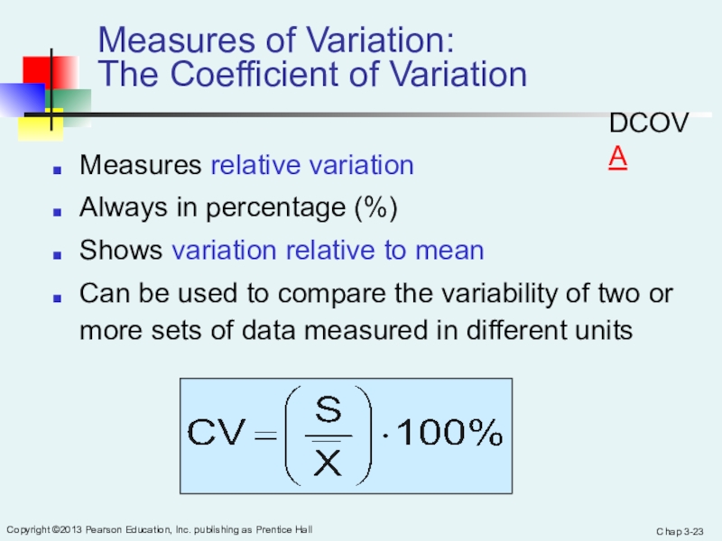
The Coefficient of Variation
Measures relative variation
Always in percentage
(%)Shows variation relative to mean
Can be used to compare the variability of two or more sets of data measured in different units
DCOVA
Слайд 24Chap 3-
Copyright ©2013 Pearson Education, Inc. publishing as Prentice Hall
Measures of Variation:
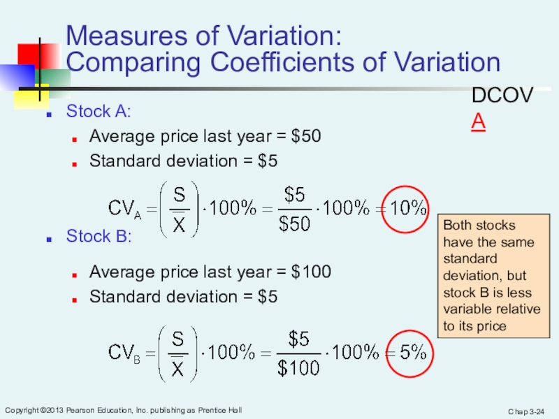
Comparing Coefficients of Variation
Stock A:
Average price last year
= $50Standard deviation = $5
Stock B:
Average price last year = $100
Standard deviation = $5
Both stocks have the same standard deviation, but stock B is less variable relative to its price
DCOVA
Слайд 25Chap 3-
Copyright ©2013 Pearson Education, Inc. publishing as Prentice Hall
Measures of Variation:
Comparing Coefficients of Variation
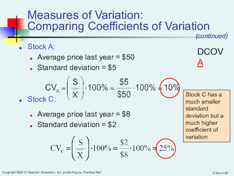
Stock A:
Average price last year
= $50Standard deviation = $5
Stock C:
Average price last year = $8
Standard deviation = $2
Stock C has a much smaller standard deviation but a much higher coefficient of variation
DCOVA
(continued)
Слайд 26Chap 3-
Copyright ©2013 Pearson Education, Inc. publishing as Prentice Hall
Locating Extreme Outliers:
Z-Score
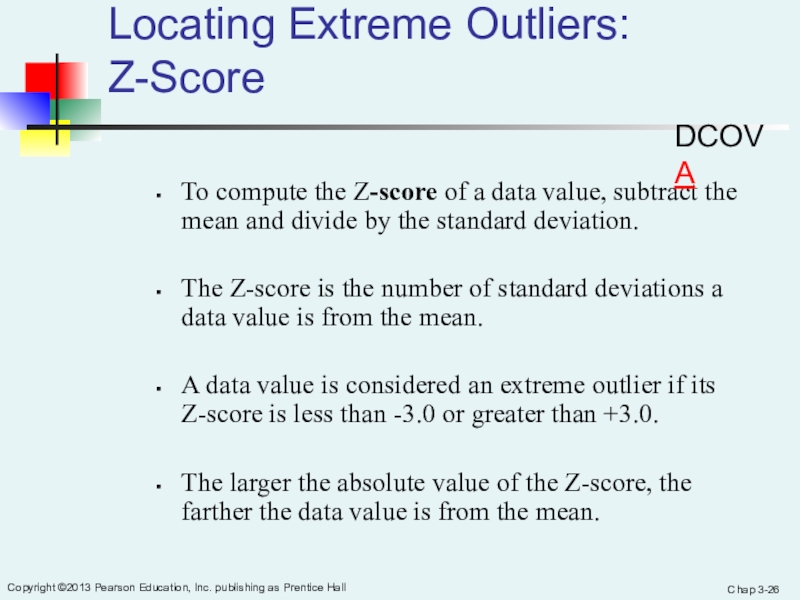
To compute the Z-score of a data value,
subtract the mean and divide by the standard deviation.The Z-score is the number of standard deviations a data value is from the mean.
A data value is considered an extreme outlier if its Z-score is less than -3.0 or greater than +3.0.
The larger the absolute value of the Z-score, the farther the data value is from the mean.
DCOVA
Слайд 27Chap 3-
Copyright ©2013 Pearson Education, Inc. publishing as Prentice Hall
Locating Extreme Outliers:
Z-Score
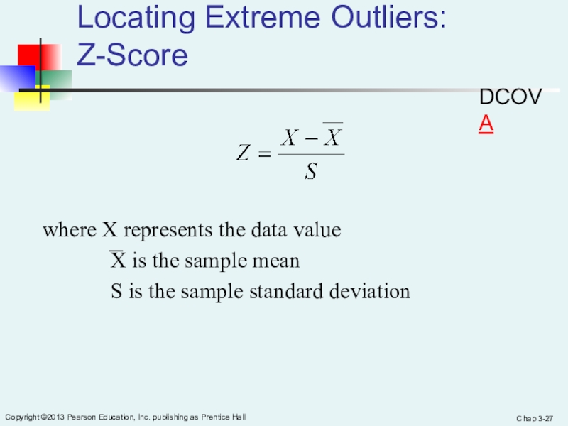
where X represents the data value
X is
the sample meanS is the sample standard deviation
DCOVA
Слайд 28Chap 3-
Copyright ©2013 Pearson Education, Inc. publishing as Prentice Hall
Locating Extreme Outliers:
Z-Score
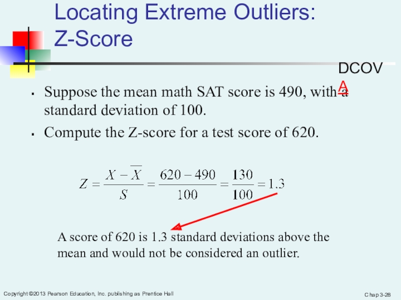
Suppose the mean math SAT score is 490,
with a standard deviation of 100.Compute the Z-score for a test score of 620.
A score of 620 is 1.3 standard deviations above the mean and would not be considered an outlier.
DCOVA
Слайд 29Chap 3-
Copyright ©2013 Pearson Education, Inc. publishing as Prentice Hall
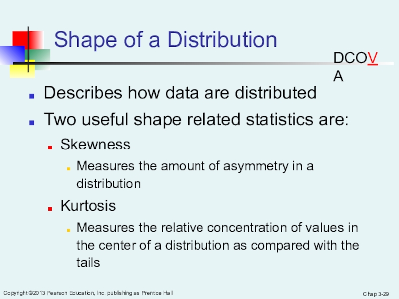
Shape of a Distribution
Describes how data are distributed
Two useful shape
related statistics are:Skewness
Measures the amount of asymmetry in a distribution
Kurtosis
Measures the relative concentration of values in the center of a distribution as compared with the tails
DCOVA
Слайд 30Chap 3-
Copyright ©2013 Pearson Education, Inc. publishing as Prentice Hall
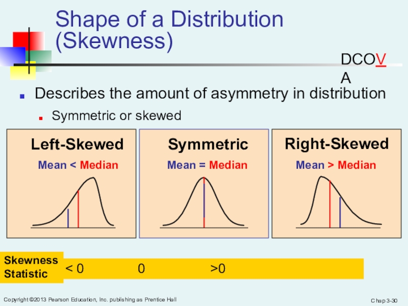
Shape of a Distribution (Skewness)
Describes the amount of asymmetry in
distributionSymmetric or skewed
Mean = Median
Mean < Median
Mean > Median
Right-Skewed
Left-Skewed
Symmetric
DCOVA
Skewness
Statistic
< 0 0 >0
Слайд 31Chap 3-
Copyright ©2013 Pearson Education, Inc. publishing as Prentice Hall
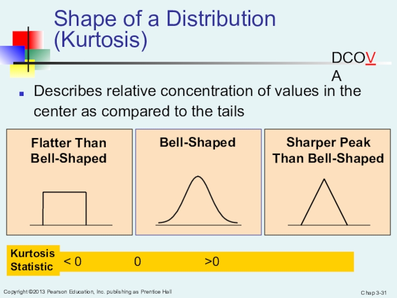
Shape of a Distribution (Kurtosis)
Describes relative concentration of values in
the center as compared to the tails
Sharper Peak
Than Bell-Shaped
Flatter Than
Bell-Shaped
Bell-Shaped
DCOVA
Kurtosis
Statistic
< 0 0 >0
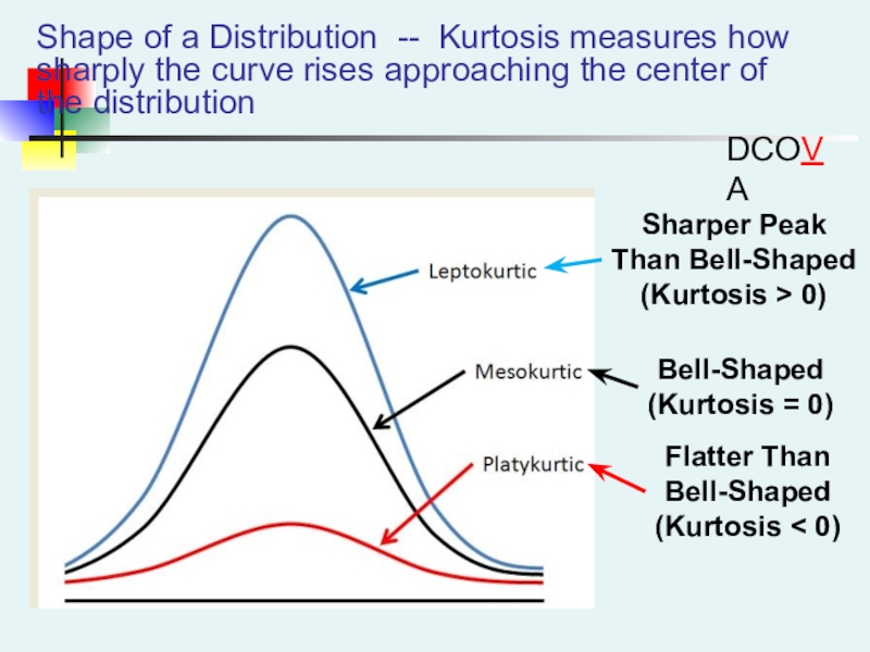
Слайд 32Shape of a Distribution -- Kurtosis measures how sharply the
curve rises approaching the center of the distribution
Sharper Peak
Than
Bell-Shaped(Kurtosis > 0)
Flatter Than
Bell-Shaped
(Kurtosis < 0)
Bell-Shaped
(Kurtosis = 0)
DCOVA
Слайд 33Chap 3-
Copyright ©2013 Pearson Education, Inc. publishing as Prentice Hall
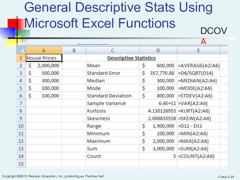
General Descriptive Stats Using Microsoft Excel Functions
DCOVA
Слайд 34Chap 3-
Copyright ©2013 Pearson Education, Inc. publishing as Prentice Hall
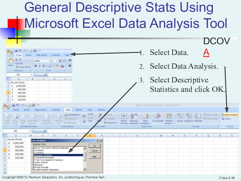
General Descriptive Stats Using Microsoft Excel Data Analysis Tool
Select Data.
Select
Data Analysis.Select Descriptive Statistics and click OK.
DCOVA
Слайд 35Chap 3-
Copyright ©2013 Pearson Education, Inc. publishing as Prentice Hall
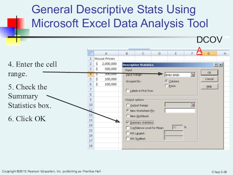
General Descriptive Stats Using Microsoft Excel Data Analysis Tool
4. Enter
the cell range.5. Check the Summary Statistics box.
6. Click OK
DCOVA
Слайд 36Chap 3-
Copyright ©2013 Pearson Education, Inc. publishing as Prentice Hall
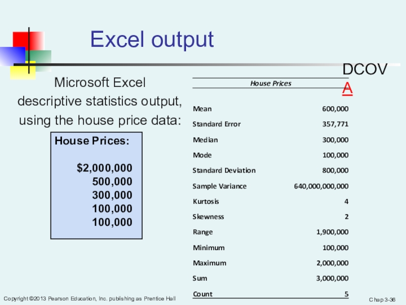
Excel output
Microsoft Excel
descriptive statistics output,
using the house price
data:House Prices:
$2,000,000
500,000
300,000
100,000
100,000
DCOVA
Слайд 37Chap 3-
Copyright ©2013 Pearson Education, Inc. publishing as Prentice Hall
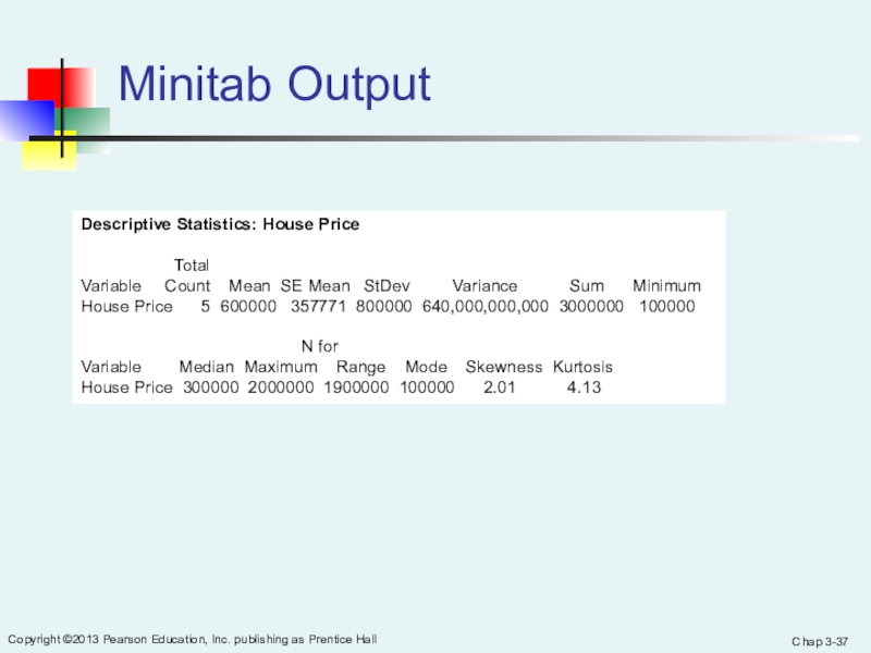
Minitab Output
Descriptive Statistics: House Price
TotalVariable Count Mean SE Mean StDev Variance Sum Minimum
House Price 5 600000 357771 800000 640,000,000,000 3000000 100000
N for
Variable Median Maximum Range Mode Skewness Kurtosis
House Price 300000 2000000 1900000 100000 2.01 4.13
Слайд 38Chap 3-
Copyright ©2013 Pearson Education, Inc. publishing as Prentice Hall
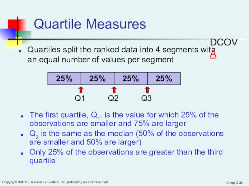
Quartile Measures
Quartiles split the ranked data into 4 segments with
an equal number of values per segmentThe first quartile, Q1, is the value for which 25% of the observations are smaller and 75% are larger
Q2 is the same as the median (50% of the observations are smaller and 50% are larger)
Only 25% of the observations are greater than the third quartile
Q1
Q2
Q3
DCOVA
Слайд 39Chap 3-
Copyright ©2013 Pearson Education, Inc. publishing as Prentice Hall
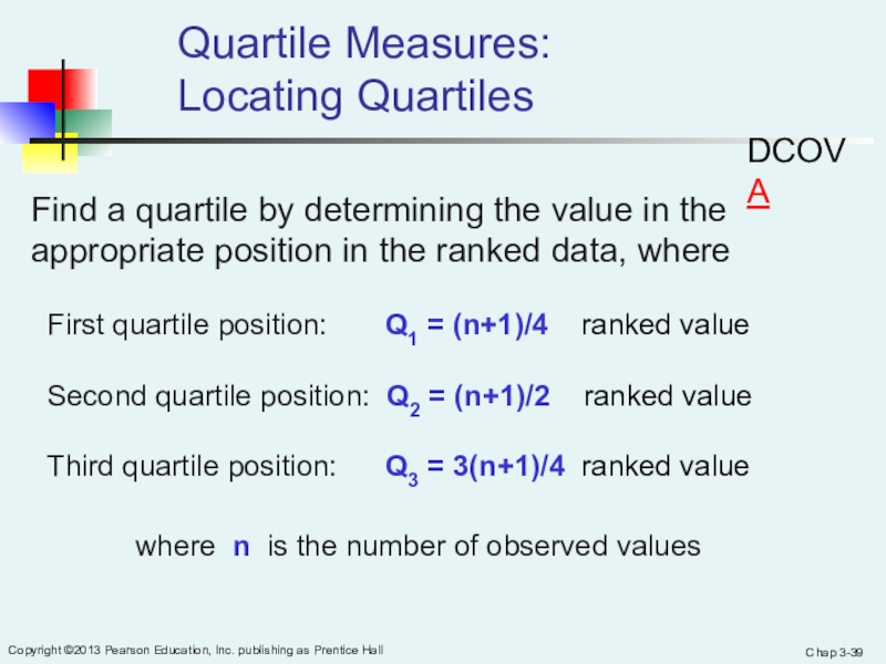
Quartile Measures:
Locating Quartiles
Find a quartile by determining the value in
the appropriate position in the ranked data, whereFirst quartile position: Q1 = (n+1)/4 ranked value
Second quartile position: Q2 = (n+1)/2 ranked value
Third quartile position: Q3 = 3(n+1)/4 ranked value
where n is the number of observed values
DCOVA
Слайд 40Chap 3-
Copyright ©2013 Pearson Education, Inc. publishing as Prentice Hall
Quartile Measures:
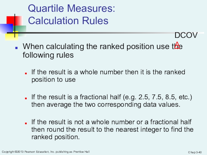
Calculation Rules
When calculating the ranked position use the following
rulesIf the result is a whole number then it is the ranked position to use
If the result is a fractional half (e.g. 2.5, 7.5, 8.5, etc.) then average the two corresponding data values.
If the result is not a whole number or a fractional half then round the result to the nearest integer to find the ranked position.
DCOVA
Слайд 41Chap 3-
Copyright ©2013 Pearson Education, Inc. publishing as Prentice Hall
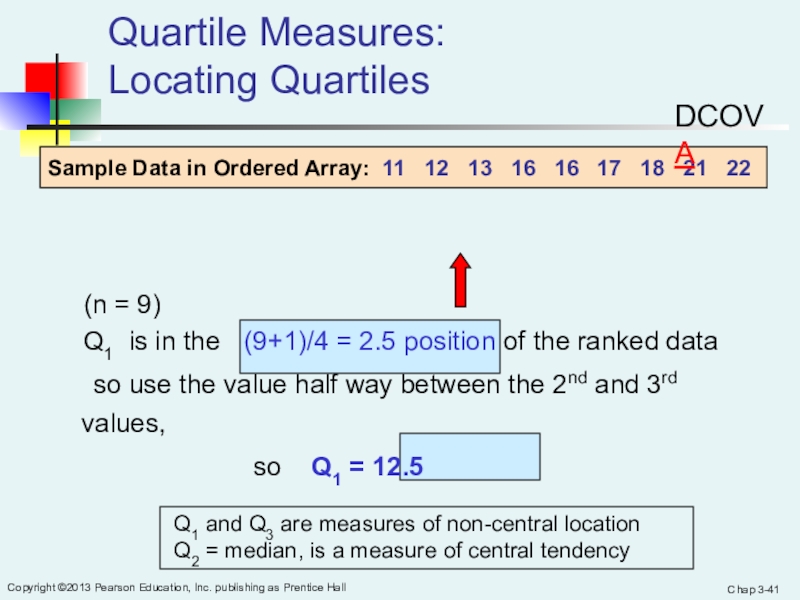
(n = 9)
Q1 is in the
(9+1)/4 = 2.5 position of the ranked dataso use the value half way between the 2nd and 3rd values,
so Q1 = 12.5
Quartile Measures:
Locating Quartiles
Sample Data in Ordered Array: 11 12 13 16 16 17 18 21 22
Q1 and Q3 are measures of non-central location
Q2 = median, is a measure of central tendency
DCOVA
Слайд 42Chap 3-
Copyright ©2013 Pearson Education, Inc. publishing as Prentice Hall
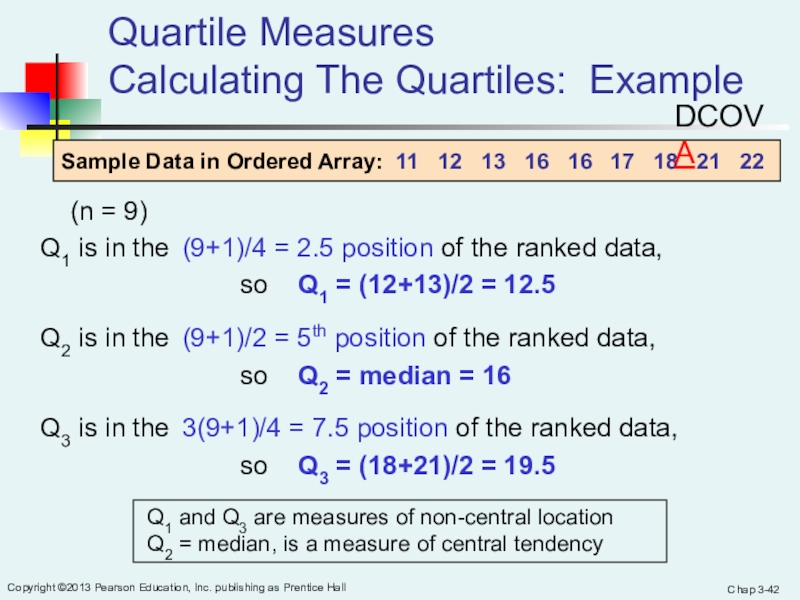
(n = 9)
Q1 is in the (9+1)/4 =
2.5 position of the ranked data,so Q1 = (12+13)/2 = 12.5
Q2 is in the (9+1)/2 = 5th position of the ranked data,
so Q2 = median = 16
Q3 is in the 3(9+1)/4 = 7.5 position of the ranked data,
so Q3 = (18+21)/2 = 19.5
Quartile Measures
Calculating The Quartiles: Example
Sample Data in Ordered Array: 11 12 13 16 16 17 18 21 22
Q1 and Q3 are measures of non-central location
Q2 = median, is a measure of central tendency
DCOVA
Слайд 43Chap 3-
Copyright ©2013 Pearson Education, Inc. publishing as Prentice Hall
Quartile Measures:
The Interquartile Range (IQR)
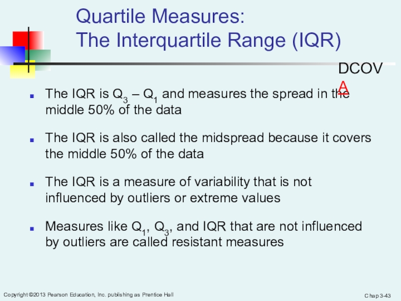
The IQR is Q3 – Q1
and measures the spread in the middle 50% of the dataThe IQR is also called the midspread because it covers the middle 50% of the data
The IQR is a measure of variability that is not influenced by outliers or extreme values
Measures like Q1, Q3, and IQR that are not influenced by outliers are called resistant measures
DCOVA
Слайд 44Chap 3-
Copyright ©2013 Pearson Education, Inc. publishing as Prentice Hall
Calculating The Interquartile Range
Median
(Q2)
X
maximum
X
minimum
Q1
Q3
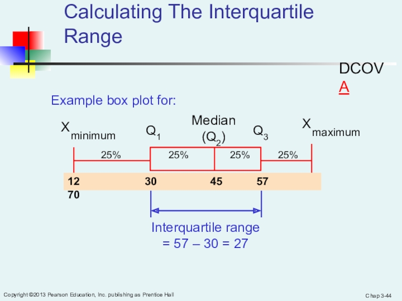
Example box plot for:
25%
25% 25% 25%12 30 45 57 70
Interquartile range
= 57 – 30 = 27
DCOVA
Слайд 45Chap 3-
Copyright ©2013 Pearson Education, Inc. publishing as Prentice Hall
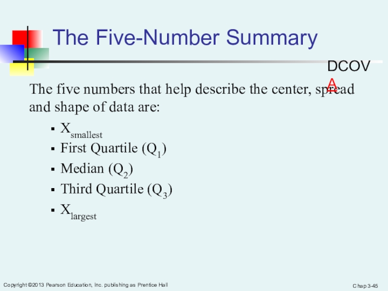
The Five-Number Summary
The five numbers that help describe the center,
spread and shape of data are:Xsmallest
First Quartile (Q1)
Median (Q2)
Third Quartile (Q3)
Xlargest
DCOVA
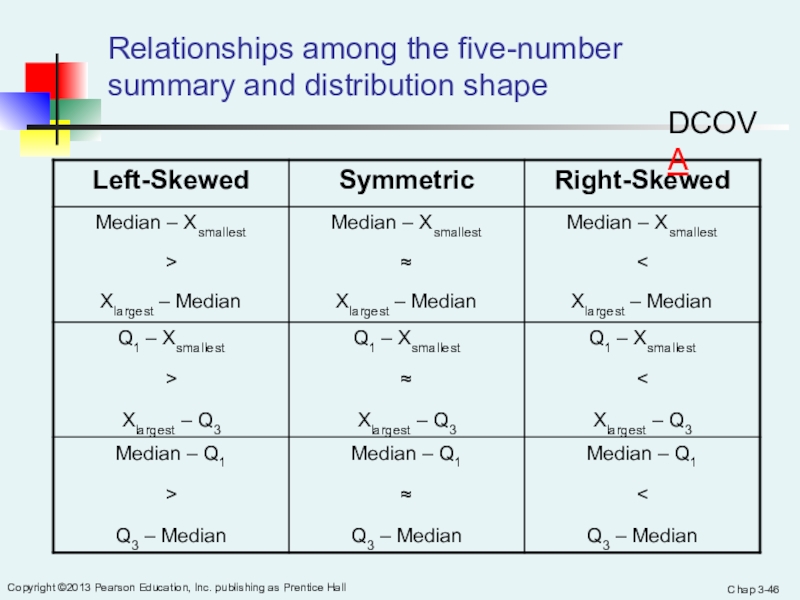
Слайд 46Chap 3-
Copyright ©2013 Pearson Education, Inc. publishing as Prentice Hall
Relationships among the five-number summary and distribution shape
DCOVA
Слайд 47Chap 3-
Copyright ©2013 Pearson Education, Inc. publishing as Prentice Hall
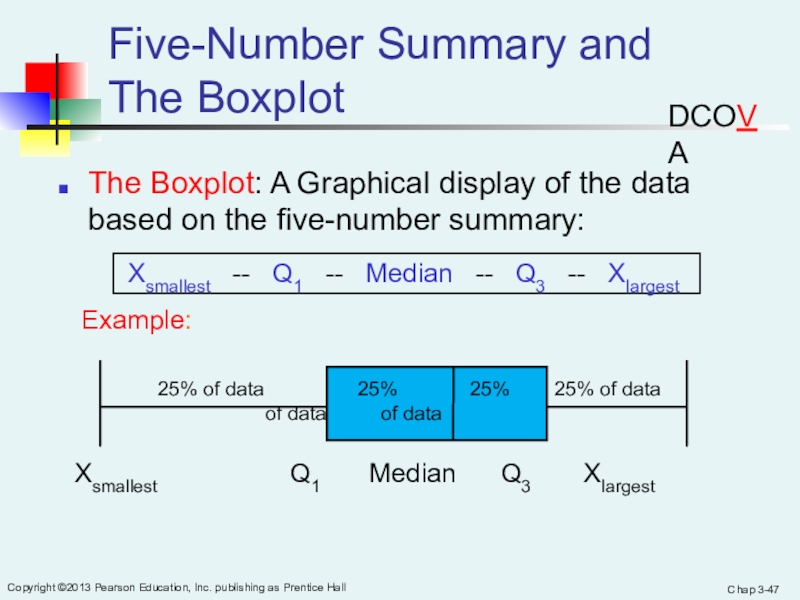
Five-Number Summary and
The Boxplot
The Boxplot: A Graphical display of the
data based on the five-number summary:Example:
Xsmallest -- Q1 -- Median -- Q3 -- Xlargest
25% of data 25% 25% 25% of data
of data of data
Xsmallest Q1 Median Q3 Xlargest
DCOVA
Слайд 48Chap 3-
Copyright ©2013 Pearson Education, Inc. publishing as Prentice Hall
Five-Number Summary:
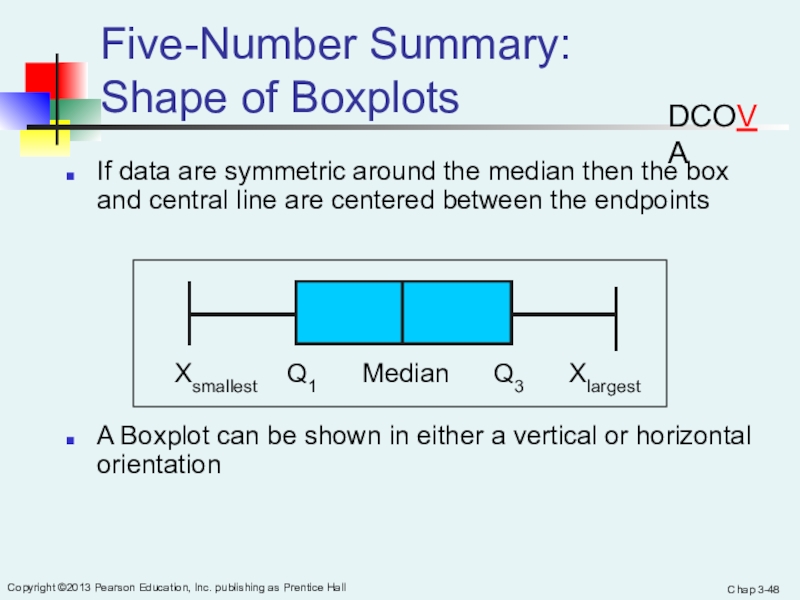
Shape of Boxplots
If data are symmetric around the median
then the box and central line are centered between the endpointsA Boxplot can be shown in either a vertical or horizontal orientation
Xsmallest Q1 Median Q3 Xlargest
DCOVA
Слайд 50Chap 3-
Copyright ©2013 Pearson Education, Inc. publishing as Prentice Hall
Distribution Shape and
The Boxplot
Right-Skewed
Left-Skewed
Symmetric
Q1
Q2
Q3
Q1
Q2
Q3
Q1
Q2
Q3
DCOVA
Слайд 52Chap 3-
Copyright ©2013 Pearson Education, Inc. publishing as Prentice Hall
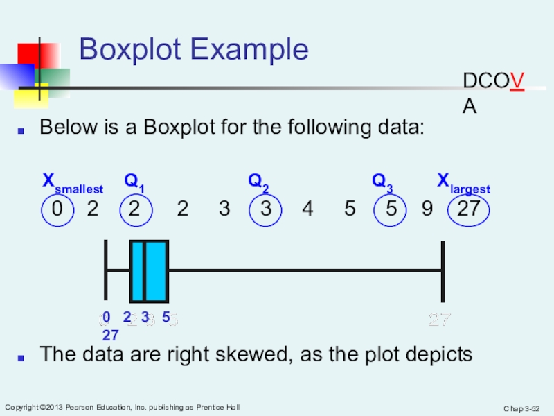
Boxplot Example
Below is a Boxplot for the following data:
0
2 2 2 3 3 4 5 5 9 27The data are right skewed, as the plot depicts
0 2 3 5 27
Xsmallest Q1 Q2 Q3 Xlargest
DCOVA
Слайд 53Chap 3-
Copyright ©2013 Pearson Education, Inc. publishing as Prentice Hall
Numerical Descriptive Measures for a Population
Descriptive statistics discussed previously described
a sample, not the population.Summary measures describing a population, called parameters, are denoted with Greek letters.
Important population parameters are the population mean, variance, and standard deviation.
DCOVA
Слайд 54Chap 3-
Copyright ©2013 Pearson Education, Inc. publishing as Prentice Hall
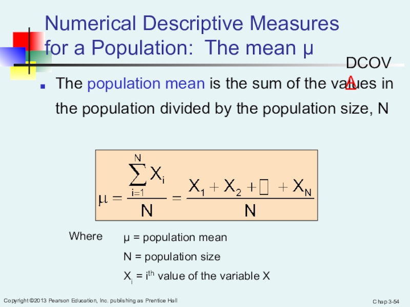
Numerical Descriptive Measures
for a Population: The mean µ
The population
mean is the sum of the values in the population divided by the population size, Nμ = population mean
N = population size
Xi = ith value of the variable X
Where
DCOVA
Слайд 55Chap 3-
Copyright ©2013 Pearson Education, Inc. publishing as Prentice Hall
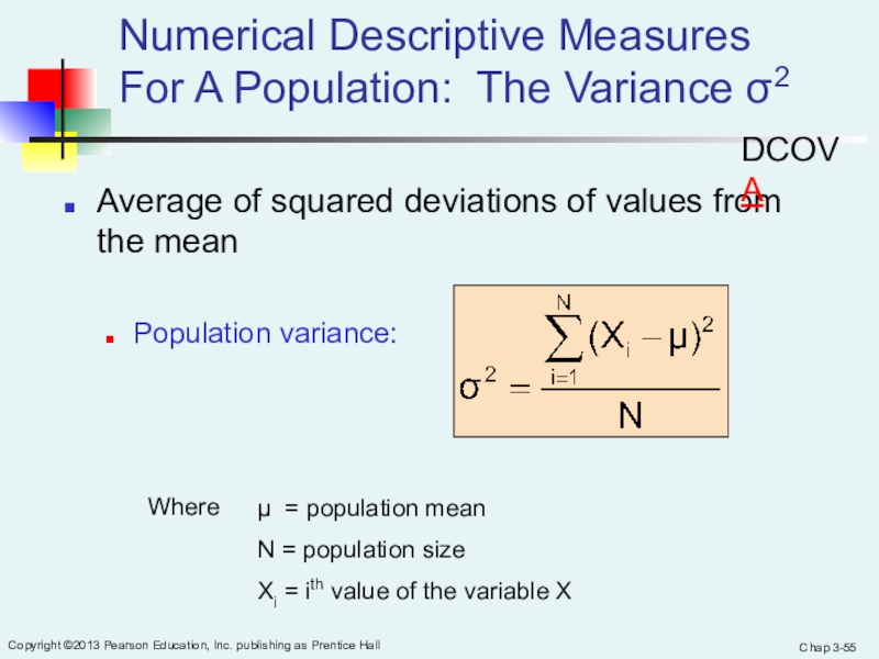
Average of squared deviations of values from the mean
Population variance:
Numerical
Descriptive Measures For A Population: The Variance σ2Where
μ = population mean
N = population size
Xi = ith value of the variable X
DCOVA
Слайд 56Chap 3-
Copyright ©2013 Pearson Education, Inc. publishing as Prentice Hall
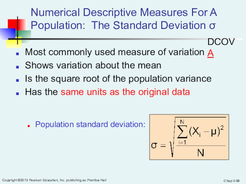
Numerical Descriptive Measures For A Population: The Standard Deviation σ
Most
commonly used measure of variationShows variation about the mean
Is the square root of the population variance
Has the same units as the original data
Population standard deviation:
DCOVA
Слайд 57Chap 3-
Copyright ©2013 Pearson Education, Inc. publishing as Prentice Hall
Sample statistics versus population parameters
DCOVA
Слайд 58Chap 3-
Copyright ©2013 Pearson Education, Inc. publishing as Prentice Hall
The empirical rule approximates the variation of data in a
bell-shaped distributionApproximately 68% of the data in a bell shaped distribution is within ± one standard deviation of the mean or
The Empirical Rule
68%
DCOVA
Слайд 59Chap 3-
Copyright ©2013 Pearson Education, Inc. publishing as Prentice Hall
Approximately 95% of the data in a bell-shaped distribution lies
within ± two standard deviations of the mean, or µ ± 2σApproximately 99.7% of the data in a bell-shaped distribution lies within ± three standard deviations of the mean, or µ ± 3σ
The Empirical Rule
99.7%
95%
DCOVA
Слайд 60Chap 3-
Copyright ©2013 Pearson Education, Inc. publishing as Prentice Hall
Using the Empirical Rule
Suppose that the variable Math SAT scores
is bell-shaped with a mean of 500 and a standard deviation of 90. Then,68% of all test takers scored between 410 and 590 (500 ± 90).
95% of all test takers scored between 320 and 680 (500 ± 180).
99.7% of all test takers scored between 230 and 770 (500 ± 270).
DCOVA
Слайд 61Chap 3-
Copyright ©2013 Pearson Education, Inc. publishing as Prentice Hall
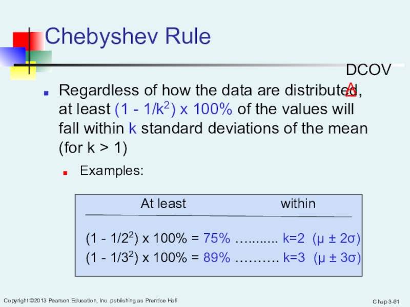
Regardless of how the data are distributed, at least (1
- 1/k2) x 100% of the values will fall within k standard deviations of the mean (for k > 1)Examples:
(1 - 1/22) x 100% = 75% …........ k=2 (μ ± 2σ)
(1 - 1/32) x 100% = 89% ………. k=3 (μ ± 3σ)
Chebyshev Rule
within
At least
DCOVA
Слайд 62Chap 3-
Copyright ©2013 Pearson Education, Inc. publishing as Prentice Hall
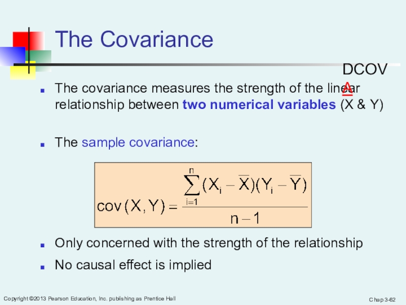
The Covariance
The covariance measures the strength of the linear relationship
between two numerical variables (X & Y)The sample covariance:
Only concerned with the strength of the relationship
No causal effect is implied
DCOVA
Слайд 63Chap 3-
Copyright ©2013 Pearson Education, Inc. publishing as Prentice Hall
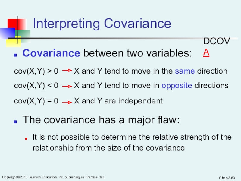
Covariance between two variables:
cov(X,Y) > 0 X
and Y tend to move in the same directioncov(X,Y) < 0 X and Y tend to move in opposite directions
cov(X,Y) = 0 X and Y are independent
The covariance has a major flaw:
It is not possible to determine the relative strength of the relationship from the size of the covariance
Interpreting Covariance
DCOVA
Слайд 64Chap 3-
Copyright ©2013 Pearson Education, Inc. publishing as Prentice Hall
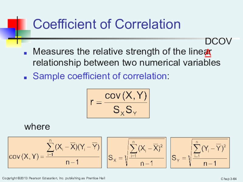
Coefficient of Correlation
Measures the relative strength of the linear relationship
between two numerical variablesSample coefficient of correlation:
where
DCOVA
Слайд 65Chap 3-
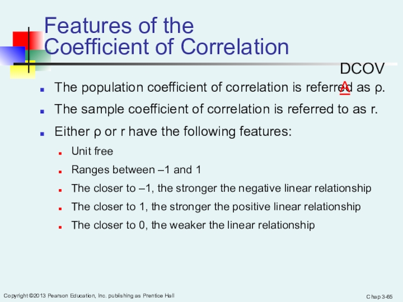
Copyright ©2013 Pearson Education, Inc. publishing as Prentice Hall
Features of the
Coefficient of Correlation
The population coefficient of correlation is
referred as ρ.The sample coefficient of correlation is referred to as r.
Either ρ or r have the following features:
Unit free
Ranges between –1 and 1
The closer to –1, the stronger the negative linear relationship
The closer to 1, the stronger the positive linear relationship
The closer to 0, the weaker the linear relationship
DCOVA
Слайд 66Chap 3-
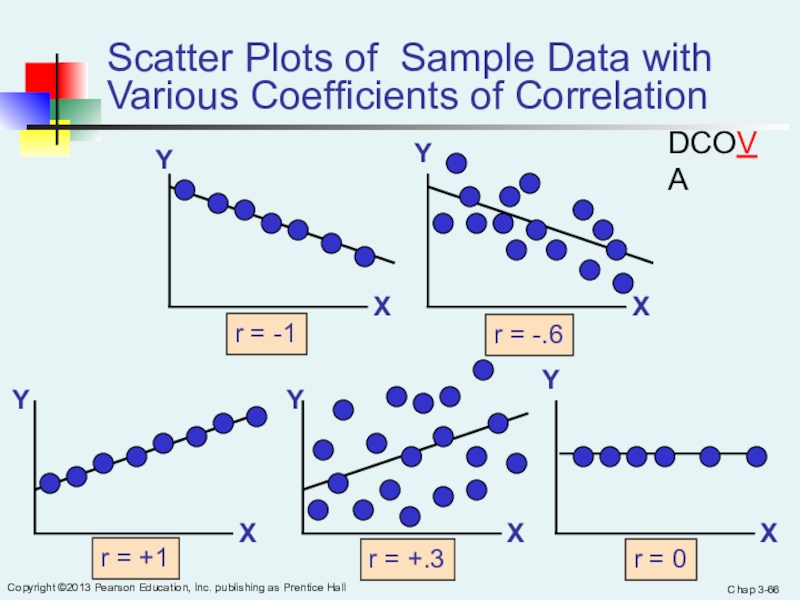
Copyright ©2013 Pearson Education, Inc. publishing as Prentice Hall
Scatter Plots of Sample Data with Various Coefficients of Correlation
Y
X
Y
X
Y
X
Y
X
r
= -1r = -.6
r = +.3
r = +1
Y
X
r = 0
DCOVA
Слайд 67Chap 3-
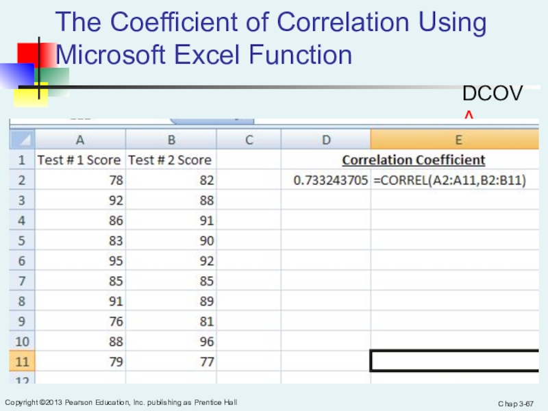
Copyright ©2013 Pearson Education, Inc. publishing as Prentice Hall
The Coefficient of Correlation Using Microsoft Excel Function
DCOVA
Слайд 68Chap 3-
Copyright ©2013 Pearson Education, Inc. publishing as Prentice Hall
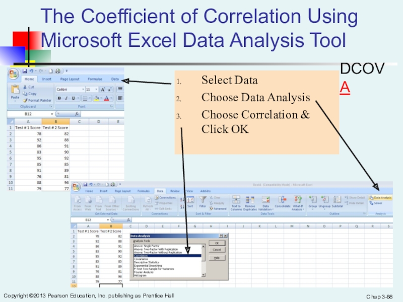
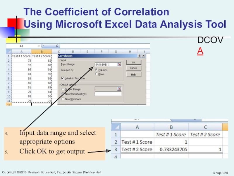
The Coefficient of Correlation Using Microsoft Excel Data Analysis Tool
Select
DataChoose Data Analysis
Choose Correlation & Click OK
DCOVA
Слайд 69Chap 3-
Copyright ©2013 Pearson Education, Inc. publishing as Prentice Hall
The Coefficient of Correlation
Using Microsoft Excel Data Analysis Tool
Input data
range and select appropriate optionsClick OK to get output
DCOVA
Слайд 70Chap 3-
Copyright ©2013 Pearson Education, Inc. publishing as Prentice Hall
Chap 3-
Interpreting the Coefficient of Correlation
Using Microsoft Excel
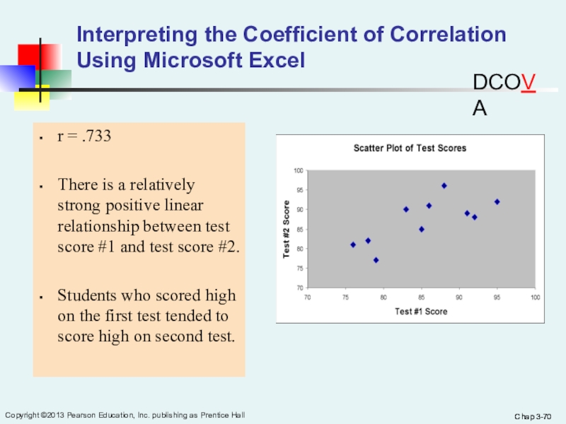
r = .733
There
is a relatively strong positive linear relationship between test score #1 and test score #2.Students who scored high on the first test tended to score high on second test.
DCOVA
Слайд 71Chap 3-
Copyright ©2013 Pearson Education, Inc. publishing as Prentice Hall
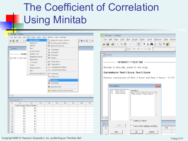
The Coefficient of Correlation Using Minitab
Слайд 72Chap 3-
Copyright ©2013 Pearson Education, Inc. publishing as Prentice Hall
Pitfalls in Numerical
Descriptive Measures
Data analysis is objective
Should report the
summary measures that best describe and communicate the important aspects of the data setData interpretation is subjective
Should be done in fair, neutral and clear manner
DCOVA
Слайд 73Chap 3-
Copyright ©2013 Pearson Education, Inc. publishing as Prentice Hall
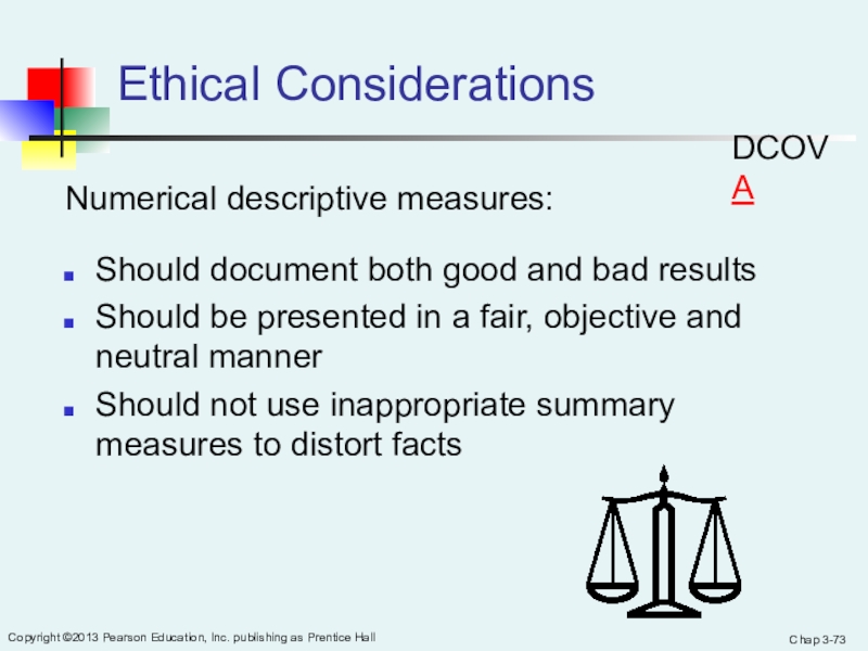
Ethical Considerations
Numerical descriptive measures:
Should document both good and bad results
Should
be presented in a fair, objective and neutral mannerShould not use inappropriate summary measures to distort facts
DCOVA
Слайд 74Chap 3-
Copyright ©2013 Pearson Education, Inc. publishing as Prentice Hall
Chapter Summary
Described measures of central tendency
Mean, median, mode
Described measures of
variationRange, interquartile range, variance and standard deviation, coefficient of variation, Z-scores
Illustrated shape of distribution
Skewness & Kurtosis
Described data using the 5-number summary
Boxplots
Слайд 75Chap 3-
Copyright ©2013 Pearson Education, Inc. publishing as Prentice Hall
Chapter Summary
Discussed covariance and correlation coefficient
Addressed pitfalls in numerical descriptive
measures and ethical considerations(continued)
Слайд 76Slide 3-
Copyright © 2011 Pearson Education, Inc.
Active Learning
Lecture Slides
For use with Classroom Response Systems
Displaying and Describing
Quantitative DataBusiness Statistics: A First Course
Слайд 77Slide 5-
Copyright © 2011 Pearson Education, Inc.
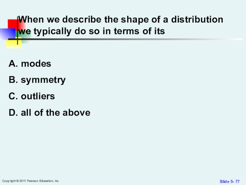
When we describe
the shape of a distribution we typically do so in
terms of itsmodes
symmetry
outliers
all of the above
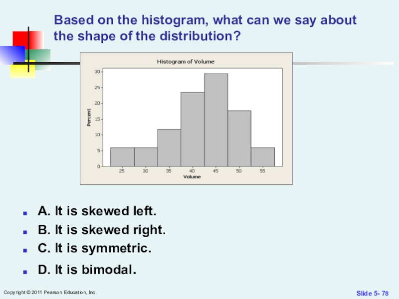
Слайд 78Based on the histogram, what can we say about the
shape of the distribution?
Slide 5-
Copyright © 2011 Pearson Education,
Inc.
A. It is skewed left.
B. It is skewed right.
C. It is symmetric.
D. It is bimodal.
Слайд 79Slide 5-
Copyright © 2011 Pearson Education, Inc.
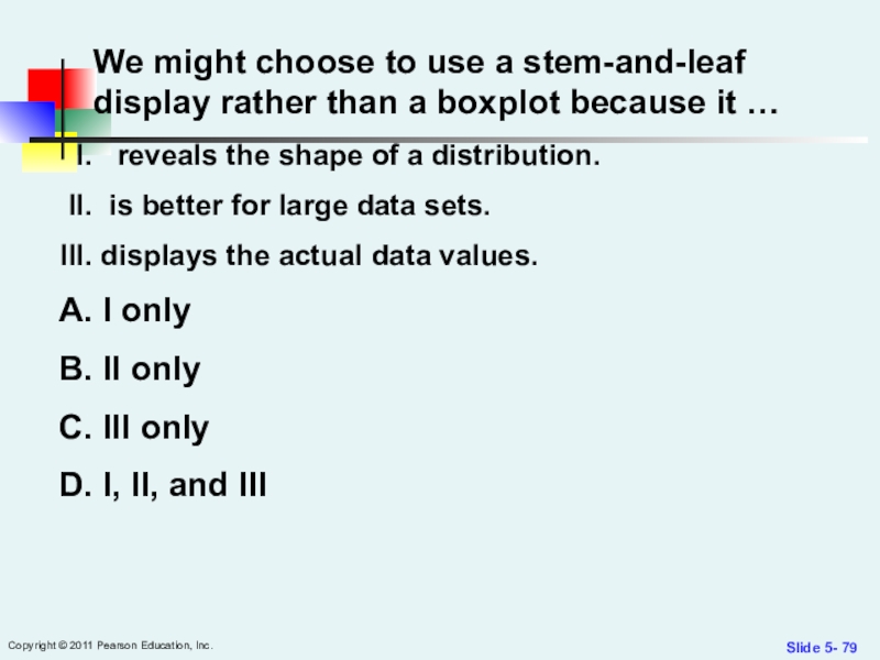
We might choose
to use a stem-and-leaf display rather than a boxplot because
it …reveals the shape of a distribution.
is better for large data sets.
displays the actual data values.
I only
II only
III only
I, II, and III
Слайд 80Slide 5-
Copyright © 2011 Pearson Education, Inc.
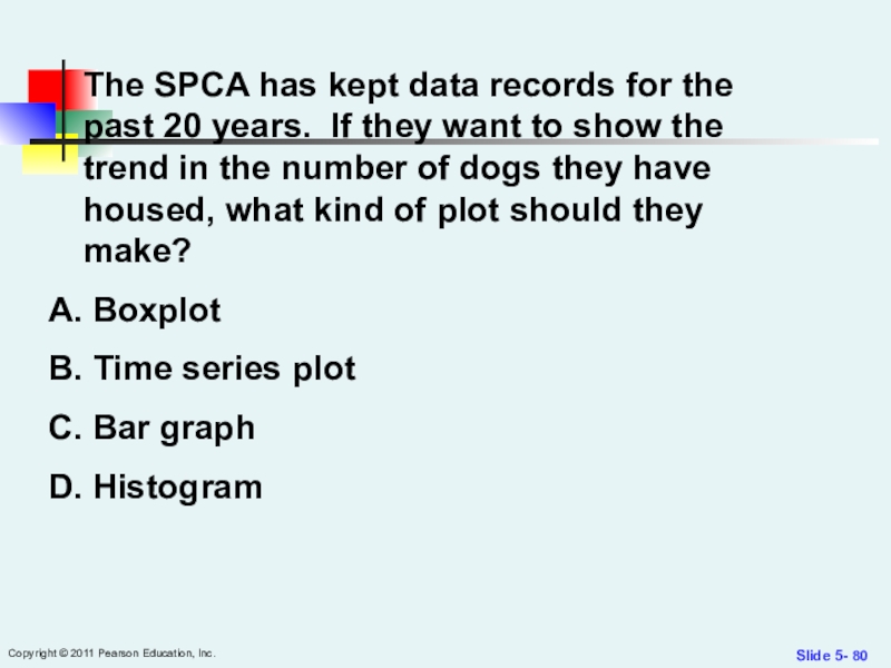
The SPCA has
kept data records for the past 20 years. If they
want to show the trend in the number of dogs they have housed, what kind of plot should they make?Boxplot
Time series plot
Bar graph
Histogram
Слайд 81Slide 5-
Copyright © 2011 Pearson Education, Inc.
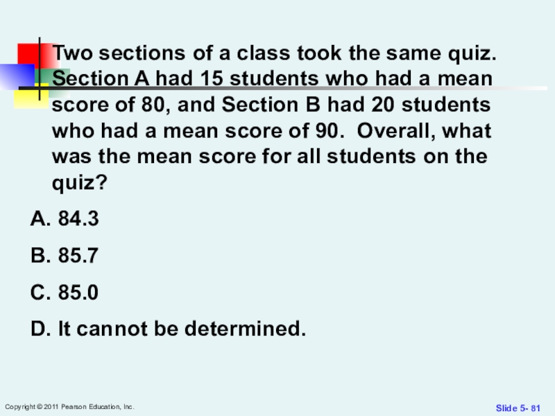
Two sections of
a class took the same quiz. Section A had 15
students who had a mean score of 80, and Section B had 20 students who had a mean score of 90. Overall, what was the mean score for all students on the quiz?84.3
85.7
85.0
It cannot be determined.
Слайд 82Slide 5-
Copyright © 2011 Pearson Education, Inc.
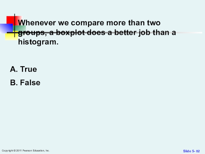
Whenever we compare
more than two groups, a boxplot does a better job
than a histogram.True
False
Слайд 83Slide 5-
Copyright © 2011 Pearson Education, Inc.
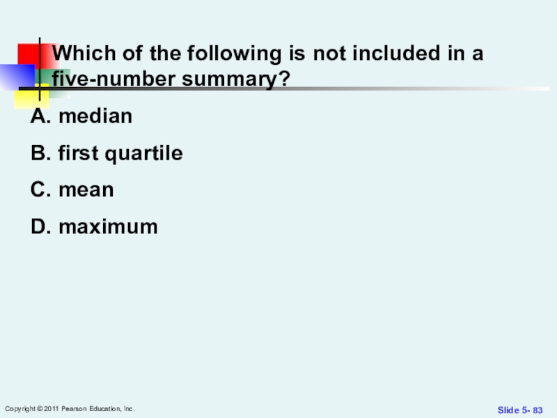
Which of the
following is not included in a five-number summary?
median
first quartilemean
maximum
Слайд 84Slide 5-
Copyright © 2011 Pearson Education, Inc.
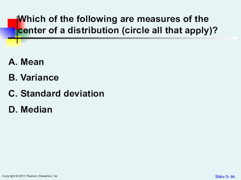
Which of the
following are measures of the center of a distribution (circle
all that apply)?Mean
Variance
Standard deviation
Median
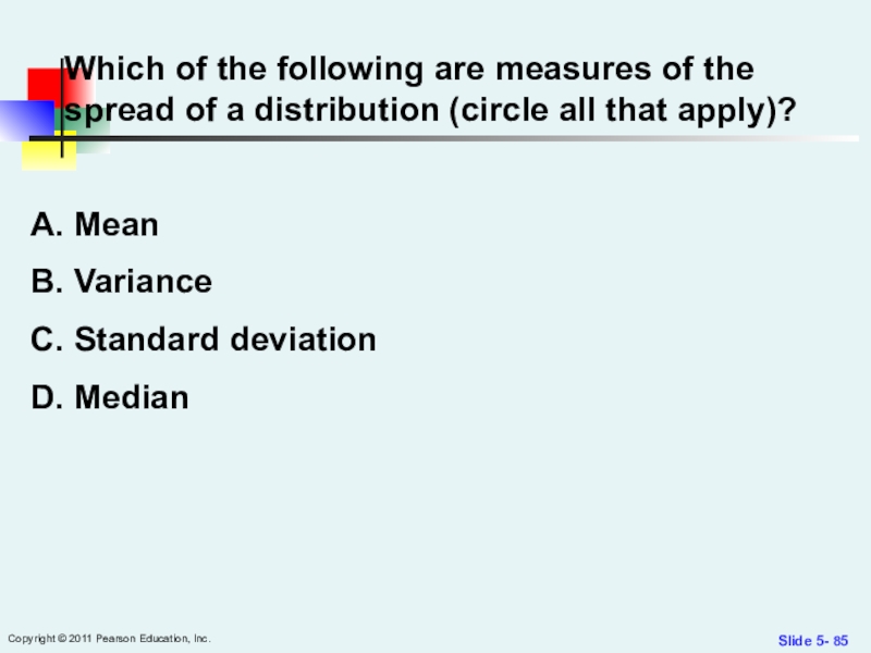
Слайд 85Slide 5-
Copyright © 2011 Pearson Education, Inc.
Which of the
following are measures of the spread of a distribution (circle
all that apply)?Mean
Variance
Standard deviation
Median
Слайд 86Slide 5-
Copyright © 2011 Pearson Education, Inc.
If you cannot
find a reason for an outlier or remove it, you
should use the mean and IQR to summarize the center and spread.True
False
