Excel

Содержание

1. Excel
2. Plan to grind up• Mean• Standard
3. Mean Enter the scores in one of
4. Standard ErrorThe formula for calculating the Standard
5. MedianThe MEDIAN function returns the median (middle
6. ModeThe Excel MODE function returns the most
7. Standard deviationUse the Excel Formula =STDEV( )
8. Sample VarianceSample Variance Excel 2013: VAR Function.
9. KurtosisKURT(number1, [number2], ...)The KURT function syntax has
10. SkewnessSKEW(number1, [number2], ...)The SKEW function syntax has
11. RangeRange = maximum value – minimum valueSo
12. Maximum=MAX (number1, [number2], ...)
13. Minimum=MIN (number1, [number2], ...)
14. SumThe SUM function, one of the math
15. CountThe COUNT function counts the number of
16. Скачать презентанцию

Plan to grind up• Mean• Standard error• Median• Mode• Standard deviation• Sample Variance• Kurtosis• Skewness• Range• Maximum• Minimum• Sum• Count

Слайды и текст этой презентации

Слайд 1Excel

Student ATAUL MUJEEB CHEEMA
Checked by AUBAKIR.E

Слайд 2Plan to grind up
• Mean• Standard error• Median• Mode• Standard

deviation• Sample Variance• Kurtosis• Skewness• Range• Maximum• Minimum• Sum• Count

Plan to grind up• Mean• Standard error• Median• Mode• Standard deviation• Sample Variance• Kurtosis• Skewness• Range•

Слайд 3Mean
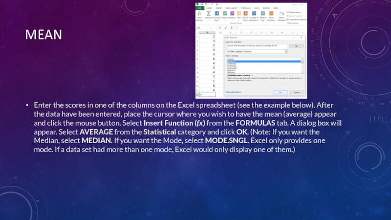
Enter the scores in one of the columns on the

Excel spreadsheet (see the example below). After the data have

been entered, place the cursor where you wish to have the mean (average) appear and click the mouse button. Select Insert Function (fx) from the FORMULAS tab. A dialog box will appear. Select AVERAGE from the Statistical category and click OK. (Note: If you want the Median, select MEDIAN. If you want the Mode, select MODE.SNGL. Excel only provides one mode. If a data set had more than one mode, Excel would only display one of them.)

Mean Enter the scores in one of the columns on the Excel spreadsheet (see the example below).

Слайд 4Standard Error
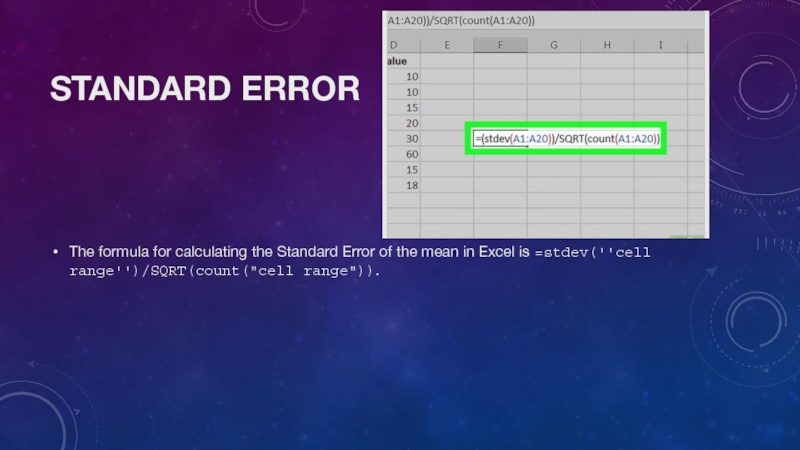
The formula for calculating the Standard Error of the

mean in Excel is =stdev(''cell range'')/SQRT(count("cell range")).

Standard ErrorThe formula for calculating the Standard Error of the mean in Excel is =stdev(''cell range'')/SQRT(count(

Слайд 5Median
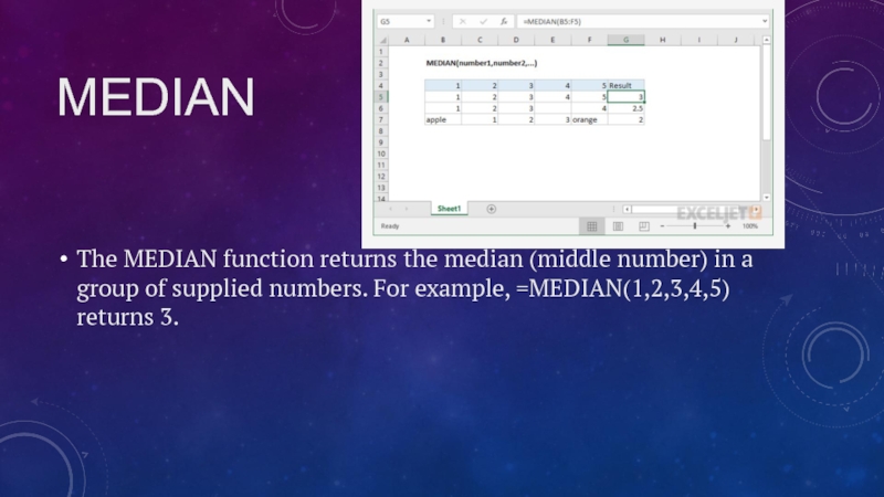
The MEDIAN function returns the median (middle number) in a

group of supplied numbers. For example, =MEDIAN(1,2,3,4,5) returns 3.

MedianThe MEDIAN function returns the median (middle number) in a group of supplied numbers. For example, =MEDIAN(1,2,3,4,5)

Слайд 6Mode
The Excel MODE function returns the most frequently occurring number in

a numeric data set. For example, =MODE(1,2,4,4,5,5,5,6) returns 5.

ModeThe Excel MODE function returns the most frequently occurring number in a numeric data set. For example, =MODE(1,2,4,4,5,5,5,6)

Слайд 7Standard deviation
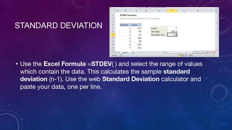
Use the Excel Formula =STDEV( ) and select the

range of values which contain the data. This calculates the

sample standard deviation (n-1). Use the web Standard Deviation calculator and paste your data, one per line.

Standard deviationUse the Excel Formula =STDEV( ) and select the range of values which contain the data.

Слайд 8Sample Variance
Sample Variance Excel 2013: VAR Function. Step 1: Type

your data into a single column. Step 3: Type “=VAR(A1:A100)”

where A1:A100 is the location of your data set (i.e. in cells A1 to A100). Press the “Enter” key to get the sample variance.

Sample VarianceSample Variance Excel 2013: VAR Function. Step 1: Type your data into a single column. Step

Слайд 9Kurtosis
KURT(number1, [number2], ...)The KURT function syntax has the following arguments:Number1,

number2, ... Number1 is required, subsequent numbers are optional. 1 to

255 arguments for which you want to calculate kurtosis. You can also use a single array or a reference to an array instead of arguments separated by commas.

KurtosisKURT(number1, [number2], ...)The KURT function syntax has the following arguments:Number1, number2, ... Number1 is required, subsequent numbers are

Слайд 10Skewness
SKEW(number1, [number2], ...)The SKEW function syntax has the following arguments:Number1,

number2, ... Number1 is required, subsequent numbers are optional. 1 to

255 arguments for which you want to calculate skewness. You can also use a single array or a reference to an array instead of arguments separated by commas.

SkewnessSKEW(number1, [number2], ...)The SKEW function syntax has the following arguments:Number1, number2, ... Number1 is required, subsequent numbers are

Слайд 11Range
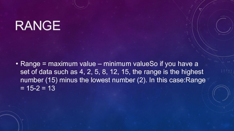
Range = maximum value – minimum valueSo if you have

a set of data such as 4, 2, 5, 8,

12, 15, the range is the highest number (15) minus the lowest number (2). In this case:Range = 15-2 = 13

RangeRange = maximum value – minimum valueSo if you have a set of data such as 4,

Слайд 12Maximum
=MAX (number1, [number2], ...)

Слайд 13Minimum
=MIN (number1, [number2], ...)

Слайд 14Sum
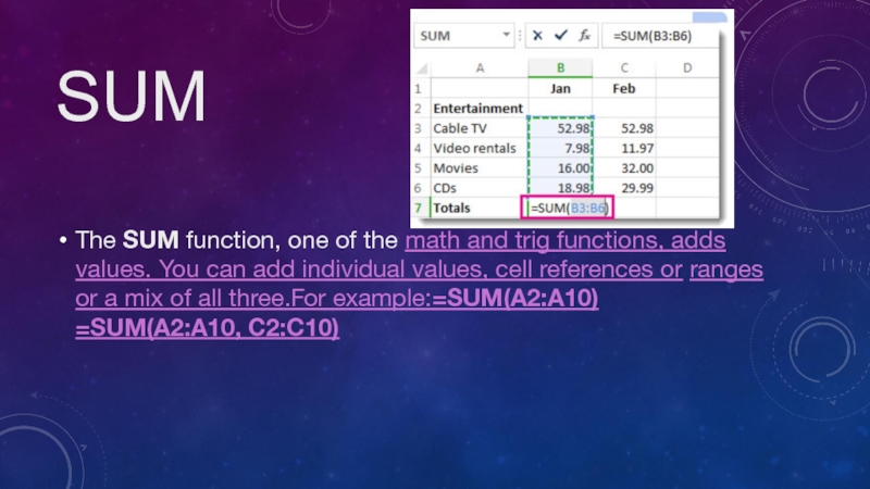
The SUM function, one of the math and trig functions,

adds values. You can add individual values, cell references or

ranges or a mix of all three.For example:=SUM(A2:A10) =SUM(A2:A10, C2:C10)

SumThe SUM function, one of the math and trig functions, adds values. You can add individual values,

Слайд 15Count
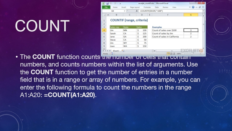
The COUNT function counts the number of cells that contain

numbers, and counts numbers within the list of arguments. Use

the COUNT function to get the number of entries in a number field that is in a range or array of numbers. For example, you can enter the following formula to count the numbers in the range A1:A20: =COUNT(A1:A20).