Разделы презентаций
- Разное
- Английский язык
- Астрономия
- Алгебра
- Биология
- География
- Геометрия
- Детские презентации
- Информатика
- История
- Литература
- Математика
- Медицина
- Менеджмент
- Музыка
- МХК
- Немецкий язык
- ОБЖ
- Обществознание
- Окружающий мир
- Педагогика
- Русский язык
- Технология
- Физика
- Философия
- Химия
- Шаблоны, картинки для презентаций
- Экология
- Экономика
- Юриспруденция
Статистическая обработка данных
Содержание
- 1. Статистическая обработка данных
- 2. Methods SectionFrom JAMA (impact factor - 47.661):In
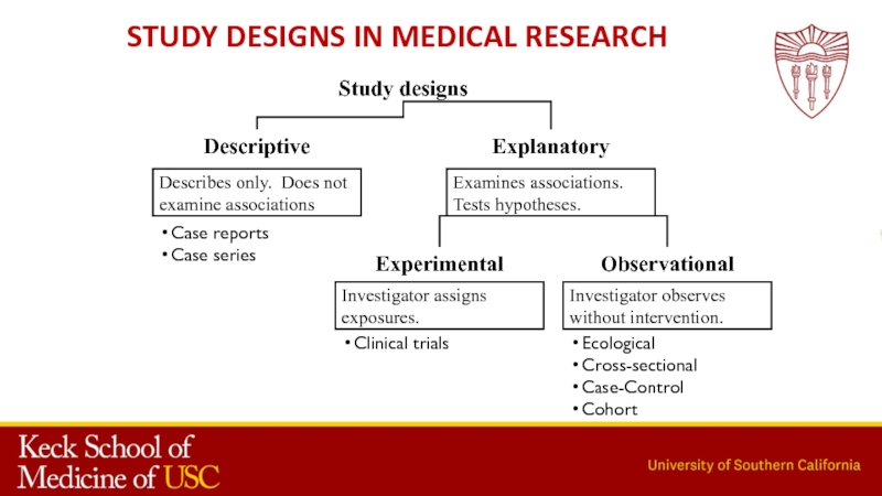
- 3. Study Designs in Medical Research
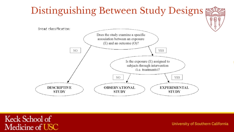
- 4. Distinguishing Between Study Designs
- 5. Common types of experiments
- 6. ExperimentIntroduce a treatment to observe its effectsMight not involve randomizationMight not even have a control group
- 7. Randomized ExperimentThe gold standard for demonstrating causalityUnits
- 8. Quasi-experimentThere is a control group, but no
- 9. Natural experiment(Not exactly an experiment because the
- 10. Correlational studyNonexperimental because nothing is manipulatedMeasure some
- 11. Even randomized experiments aren’t perfect Experimental conditions
- 12. Populations
- 13. Population vs. SamplePopulationDescribed using population parametersUsually represented
- 14. Types of Data (Variables)Categorical Nominal-mutually exclusive-no natural
- 15. Types of Data (Variables)Categorical Nominal-mutually exclusive-no natural order(qualitative)Ordinal-mutually exclusive-orderedContinuous-countable-takes any value-magnitude of value importantDichotomous
- 16. HistogramsKnow how to interpret a histogram, i.e.,
- 17. Measures of Central Tendency Mean: what’s commonly
- 18. Measures of Variability (Dispersion)
- 19. Слайд 19
- 20. CD4 count (Numerical data)One sample meanCD4Mean change
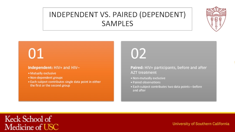
- 21. Independent vs. paired (dependent) samples
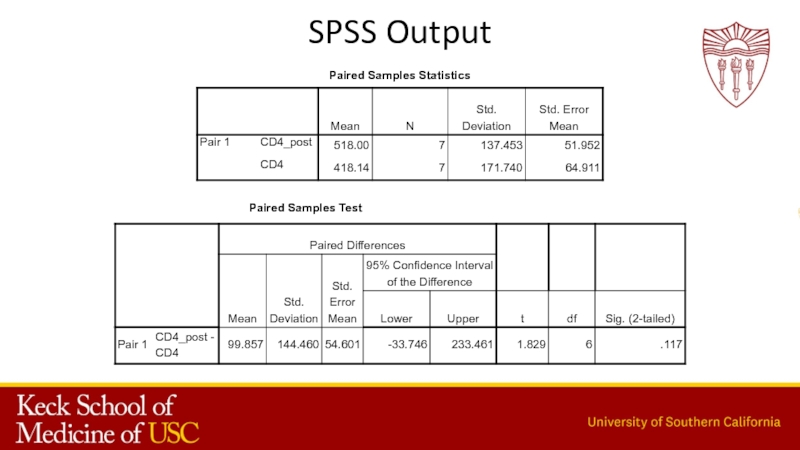
- 22. SPSS Output
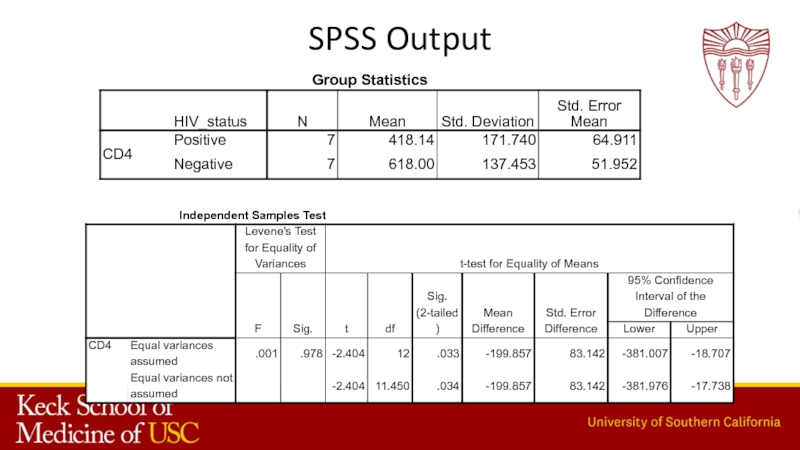
- 23. SPSS Output
- 24. Слайд 24
- 25. Слайд 25
- 26. Слайд 26
- 27. What is correlation? Correlation captures the extent to
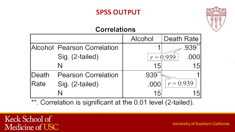
- 28. r = 0.939r = 0.939SPSS output
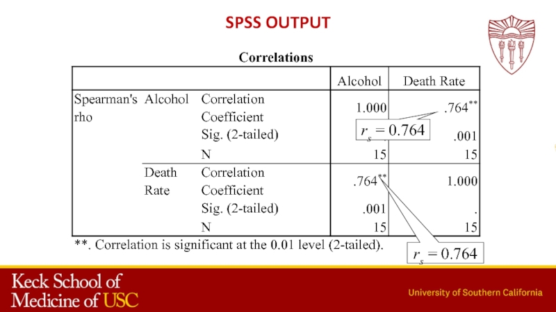
- 29. SPSS outputrs = 0.764rs = 0.764
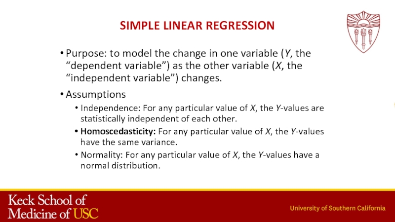
- 30. Simple linear regression Purpose: to model the
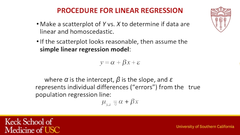
- 31. Procedure for linear regressionMake a scatterplot of
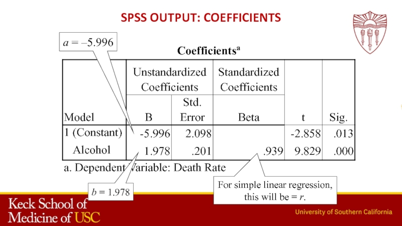
- 32. a = –5.996b = 1.978SPSS output: CoefficientsFor simple linear regression, this will be = r.
- 33. Multilevel Structured Data Multilevel data frequently encountered
- 34. Example of Multilevel Data in Prevention Research
- 35. Missing Data Data are missing on some
- 36. Missing Data: Methods to Deal with Missing
- 37. Methods Section OutlineParticipants and ProceduresMeasuresData Analysis
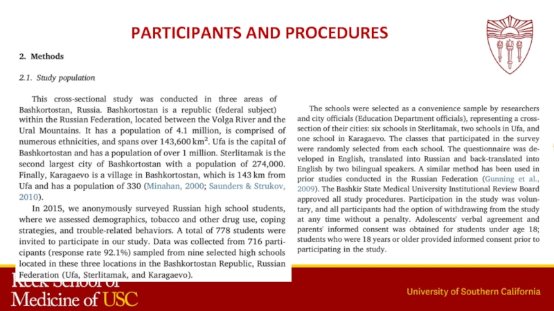
- 38. Participants and Procedures
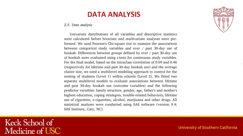
- 39. Data Analysis
- 40. Q/A Session
- 41. Arthur Galimov e-mail: galimov@usc.edu IG: ar_galimov
- 42. Скачать презентанцию
Methods SectionFrom JAMA (impact factor - 47.661):In the Methods section, describe statistical methods with enough detail to enable a knowledgeable reader with access to the original data to reproduce the reported
Слайды и текст этой презентации
Слайд 6Experiment
Introduce a treatment to observe its effects
Might not involve randomization
Might
not even have a control group
Слайд 7Randomized Experiment
The gold standard for demonstrating causality
Units (people, animals, groups,
etc.) are randomly assigned to receive either treatment or control.
If
the sample is large enough, we can assume that on the average, everything else about the two groups is similar because the two groups were randomly selected.So any difference between the two groups after the experiment must be due to the treatment.
Слайд 8Quasi-experiment
There is a control group, but no random assignment to
treatment vs. control
Usually happens because it’s impossible or unethical to
do random assignmentAssignment to conditions occurs by self-selection (some people choose to smoke or exercise or join a program)
Example: effects of a new health media campaign that’s introduced in one community but not others
The main problem is that the groups are different in other ways (people who become smokers have different demographics and genetics)
Слайд 9Natural experiment
(Not exactly an experiment because the experimenter didn’t manipulate
the cause, but the cause occurred)
Compare a group that experienced
a cause with a group that didn’t(Or compare the same group before and after the cause)
Examples: effect of a natural disaster, effect of a policy change
Слайд 10Correlational study
Nonexperimental because nothing is manipulated
Measure some variables and see
if there’s a mathematical relationship between them
Results can be consistent
with causality, but they can’t prove causalityСлайд 11Even randomized experiments aren’t perfect
Experimental conditions are usually artificial
They’re
conducted in one particular time and place – might not
generalize to other times or placesBut we usually want to generalize the findings to other times and places
Cronbach: we usually want to generalize to other UTOS – units, treatments, observations (outcomes), and settings
Слайд 13Population vs. Sample
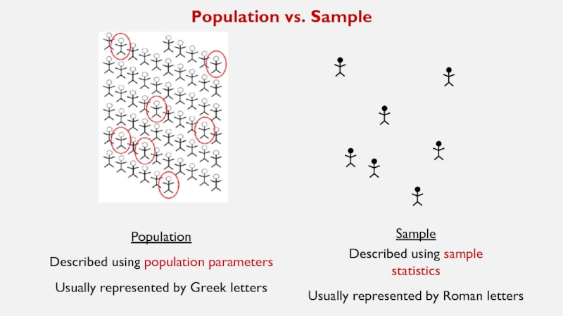
Population
Described using population parameters
Usually represented by Greek letters
Sample
Described
using sample
statistics
Usually represented by Roman letters
Слайд 14Types of Data (Variables)
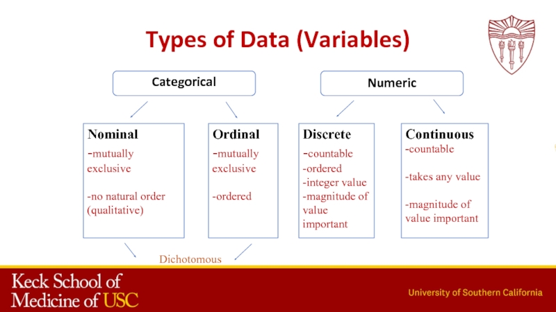
Categorical
Nominal
-mutually exclusive
-no natural order
(qualitative)
Ordinal
-mutually exclusive
-ordered
Numeric
Discrete
-countable
-ordered
-integer value
-magnitude
of value important
Continuous
-countable
-takes any value
-magnitude of value important
Dichotomous
Слайд 15Types of Data (Variables)
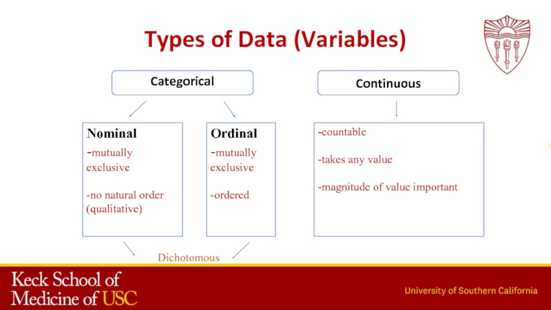
Categorical
Nominal
-mutually exclusive
-no natural order
(qualitative)
Ordinal
-mutually exclusive
-ordered
Continuous
-countable
-takes any
value
-magnitude of value important
Dichotomous
Слайд 16Histograms
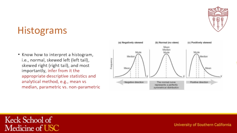
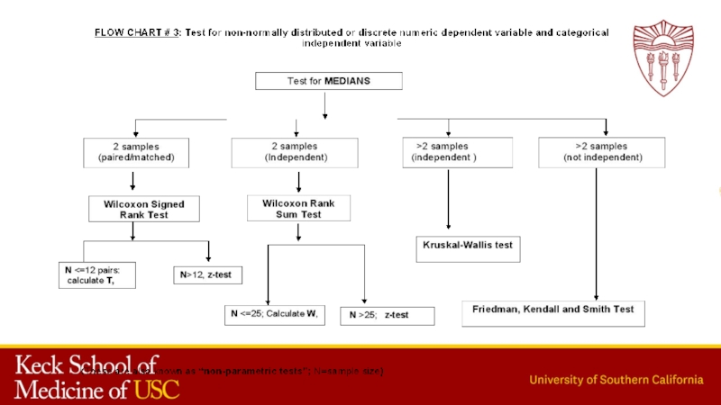
Know how to interpret a histogram, i.e., normal, skewed left
(left tail), skewed right (right tail), and most importantly, infer
from it the appropriate descriptive statistics and analytical method, e.g., mean vs median, parametric vs. non-parametricСлайд 17Measures of Central Tendency
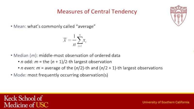
Mean: what’s commonly called “average”
Median (m):
middle-most observation of ordered data
n odd: m = the (n
+ 1)/2-th largest observationn even: m = average of the (n/2)-th and (n/2 + 1)-th largest observations
Mode: most frequently occurring observation(s)
Слайд 20CD4 count (Numerical data)
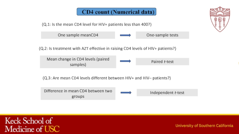
One sample meanCD4
Mean change in CD4 levels
(paired samples)
Difference in mean CD4 between two groups
Independent t-test
Paired
t-testOne-sample tests
(Q.1: Is the mean CD4 level for HIV+ patients less than 400?)
(Q.2: Is treatment with AZT effective in raising CD4 levels of HIV+ patients?)
(Q.3: Are mean CD4 levels different between HIV+ and HIV– patients?)
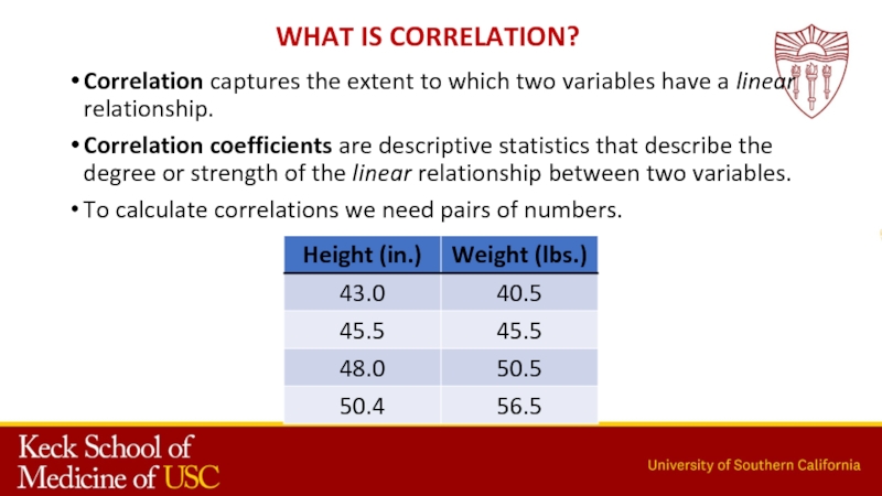
Слайд 27What is correlation?
Correlation captures the extent to which two variables
have a linear relationship.
Correlation coefficients are descriptive statistics that
describe the degree or strength of the linear relationship between two variables.To calculate correlations we need pairs of numbers.
Слайд 30Simple linear regression
Purpose: to model the change in one
variable (Y, the “dependent variable”) as the other variable (X,
the “independent variable”) changes.Assumptions
Independence: For any particular value of X, the Y-values are statistically independent of each other.
Homoscedasticity: For any particular value of X, the Y-values have the same variance.
Normality: For any particular value of X, the Y-values have a normal distribution.
Слайд 31Procedure for linear regression
Make a scatterplot of Y vs. X
to determine if data are linear and homoscedastic.
If the
scatterplot looks reasonable, then assume the simple linear regression model:where is the intercept, is the slope, and represents individual differences (“errors”) from the true population regression line:
Слайд 33Multilevel Structured Data
Multilevel data frequently encountered in social sciences
research refer to data which contain multilevel (hierarchical or nested)
structure.Multilevel structure indicates that data to be analyzed were obtained from units (e.g., individual) which are nested within higher level units (e.g., groups or clusters).
Слайд 34Example of Multilevel Data in Prevention Research
In school-based substance
use prevention research, schools are usually the units of assignment
to experimental conditions (program or control).Data are then collected from both student (micro) and school (macro) levels
student (micro) and
school (macro) levels
to evaluate program effect.
Слайд 35Missing Data
Data are missing on some variables for some
observations.
Three goals of missing data handling
Minimize bias
Maximize
use of available information Get good estimates of uncertainty (get accurate estimates of standard error, CI, p value)
Not a goal: imputed values “close” to real values
Слайд 36Missing Data: Methods to Deal with Missing
Listwise Deletion: Delete
cases with any missing on the variables being analyzed.
Missing
replacement by imputation: Mean replacement:
using variable mean or group mean
will not affect mean, but reduce variance
Regression approach
predicting the missing value on one variable with scores on other variables
Multiple imputation
Sensitivity analysis
complete cases vs. missing replacement
