Разделы презентаций
- Разное
- Английский язык
- Астрономия
- Алгебра
- Биология
- География
- Геометрия
- Детские презентации
- Информатика
- История
- Литература
- Математика
- Медицина
- Менеджмент
- Музыка
- МХК
- Немецкий язык
- ОБЖ
- Обществознание
- Окружающий мир
- Педагогика
- Русский язык
- Технология
- Физика
- Философия
- Химия
- Шаблоны, картинки для презентаций
- Экология
- Экономика
- Юриспруденция
Lecture 9
Содержание
- 1. Lecture 9
- 2. The steps involved in Business AnalysisStep 1
- 3. Learning ObjectivesAt the conclusion of this lecture
- 4. ValuationIs the process of converting the forecast
- 5. RevisionLast lecture we looked at 2 valuation
- 6. Valuation Using MultiplesPick a ratio Pick a
- 7. Discounted Dividend ModelDDM problem – dividends not
- 8. EarningsAccountants and analysts focus on earningsEarnings in
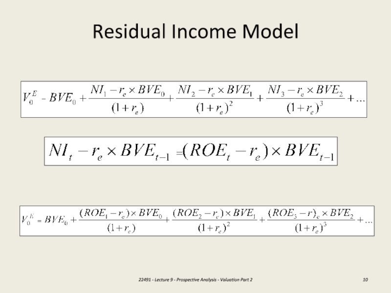
- 9. Residual Income ModelNormal Earnings Capitalised Abnormal Earnings (Residual
- 10. Residual Income Model22491 - Lecture 9 - Prospective Analysis - Valuation Part 2
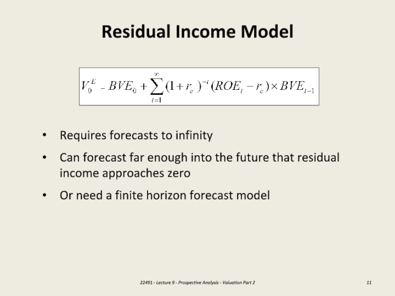
- 11. Residual Income ModelRequires forecasts to infinityCan forecast
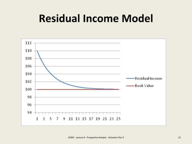
- 12. Residual Income Model22491 - Lecture 9 - Prospective Analysis - Valuation Part 2
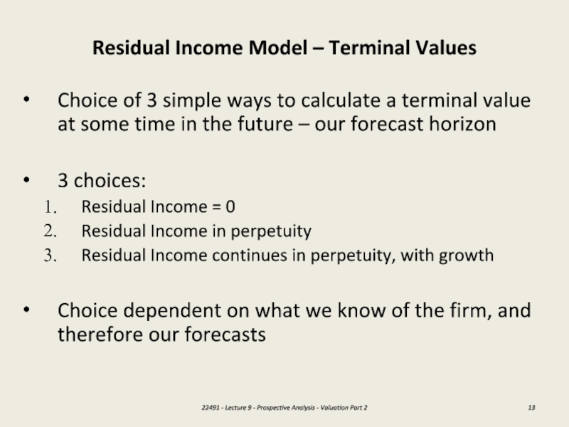
- 13. Residual Income Model – Terminal ValuesChoice of
- 14. Residual Income Model– steps in valuationForecast CSP
- 15. 1. Residual Income Model: AE = 0Why
- 16. 1. Residual Income Model: AE = 022491
- 17. Nursing Home Limited - Workings22491 - Lecture 9 - Prospective Analysis - Valuation Part 2
- 18. 2. Residual Income Model: AE continues
- 19. 2. Residual Income Model: AE continues in
- 20. 3. Residual Income Model: AE continues with
- 21. 3. Residual Income Model: AE continues
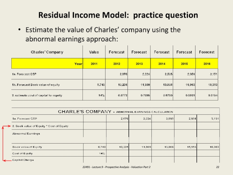
- 22. Residual Income Model: practice questionEstimate the value
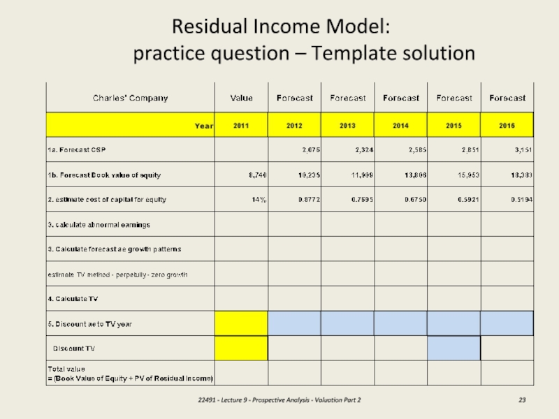
- 23. Residual Income Model: practice question –
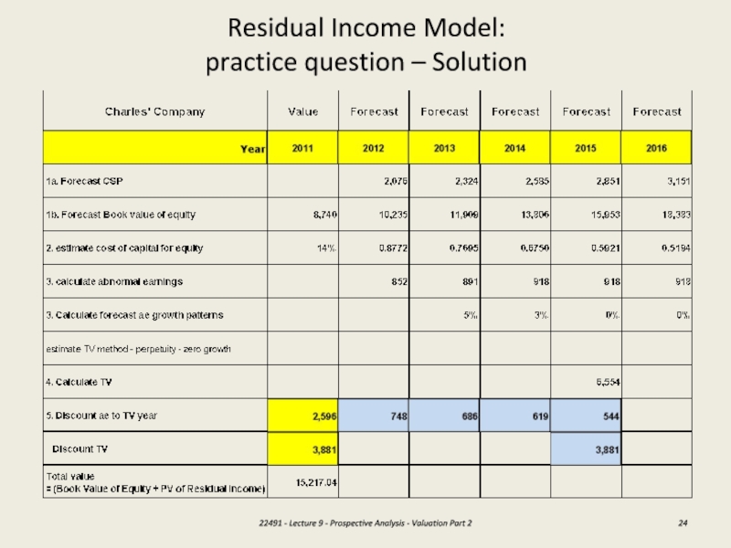
- 24. Residual Income Model: practice question –
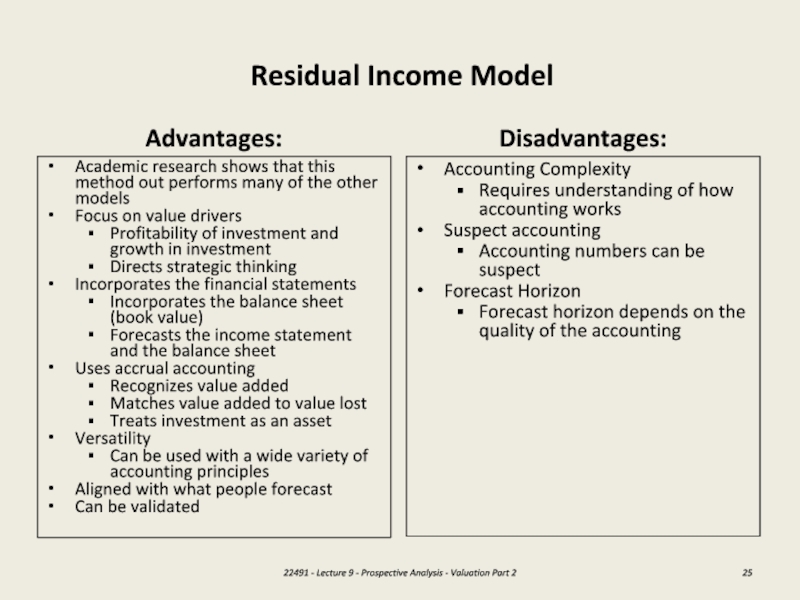
- 25. Residual Income ModelAdvantages:Academic research shows that this
- 26. Residual Operating Income Model (RIM Modified)Residual
- 27. Residual Operating Income ModelTherefore - can also
- 28. Residual OPERATING Income ModelUnder the discounted abnormal
- 29. Residual Operating Income ModelGives the same result
- 30. Residual Operating Income Model - stepsForecast NOPAT
- 31. Residual Operating Income Model - questionEstimate the
- 32. Residual OPERATING Income Model – Solution Template22491
- 33. Residual OPERATING Income Model - solution22491 - Lecture 9 - Prospective Analysis - Valuation Part 2
- 34. Free Cash Flow (DCF) ModelSimilar to the
- 35. Also forecasts over an infinite horizon: need
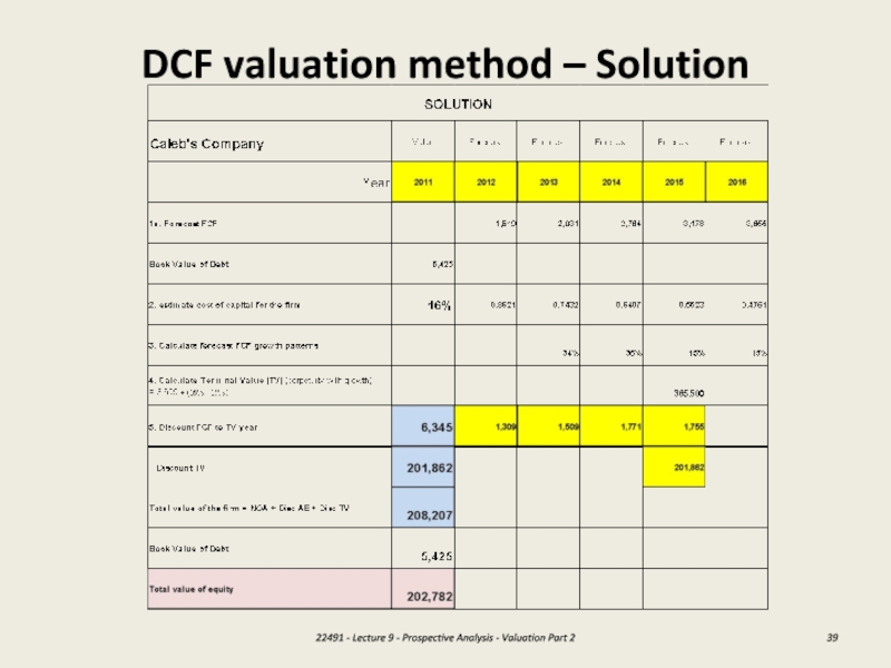
- 36. DCF valuation method - stepsForecast free cash
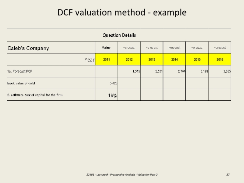
- 37. DCF valuation method - example22491 - Lecture 9 - Prospective Analysis - Valuation Part 2
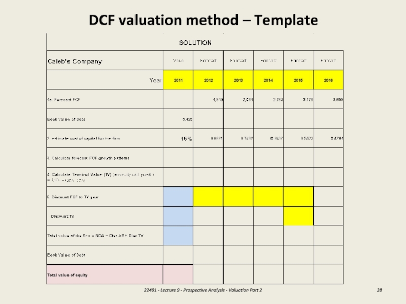
- 38. DCF valuation method – Template22491 - Lecture 9 - Prospective Analysis - Valuation Part 2
- 39. DCF valuation method – Solution22491 - Lecture 9 - Prospective Analysis - Valuation Part 2
- 40. What are the problems with DCF?Cash flow
- 41. DCF AnalysisAdvantagesEasy concept: cash flows are “real” and
- 42. Comparing the models – DDM, DCF and
- 43. Comparing the models – DDM, DCF and
- 44. SummaryValuation converts forecasts of performance into approximated
- 45. Скачать презентанцию
Слайды и текст этой презентации
Слайд 1Lecture 9
Prospective Analysis – Valuation theory and concepts (part 2)
Chapter
7 – Palepu, Healy & Peek IFRS Edition
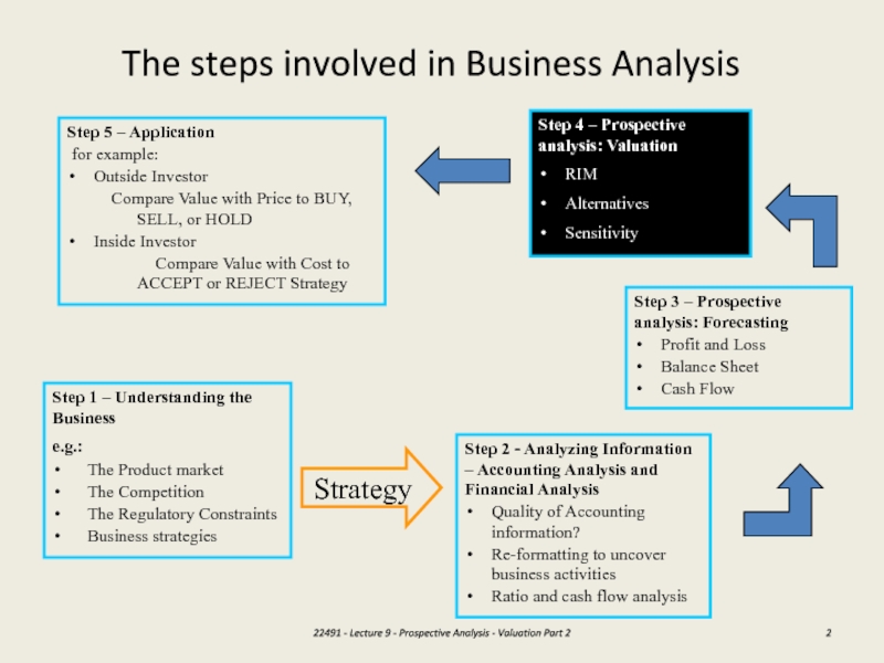
Слайд 2The steps involved in Business Analysis
Step 1 – Understanding the
Business
e.g.:
The Product market
The Competition
The Regulatory Constraints
Business strategies
Step 2 - Analyzing
Information – Accounting Analysis and Financial AnalysisQuality of Accounting information?
Re-formatting to uncover business activities
Ratio and cash flow analysis
Step 3 – Prospective analysis: Forecasting
Profit and Loss
Balance Sheet
Cash Flow
Step 4 – Prospective analysis: Valuation
RIM
Alternatives
Sensitivity
Step 5 – Application
for example:
Outside Investor
Compare Value with Price to BUY, SELL, or HOLD
Inside Investor
Compare Value with Cost to ACCEPT or REJECT Strategy
Strategy
22491 - Lecture 9 - Prospective Analysis - Valuation Part 2
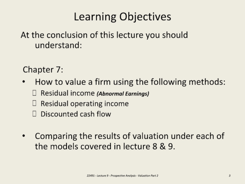
Слайд 3Learning Objectives
At the conclusion of this lecture you should understand:
Chapter 7:
How to value a firm using the following methods:
Residual
income (Abnormal Earnings)Residual operating income
Discounted cash flow
Comparing the results of valuation under each of the models covered in lecture 8 & 9.
22491 - Lecture 9 - Prospective Analysis - Valuation Part 2
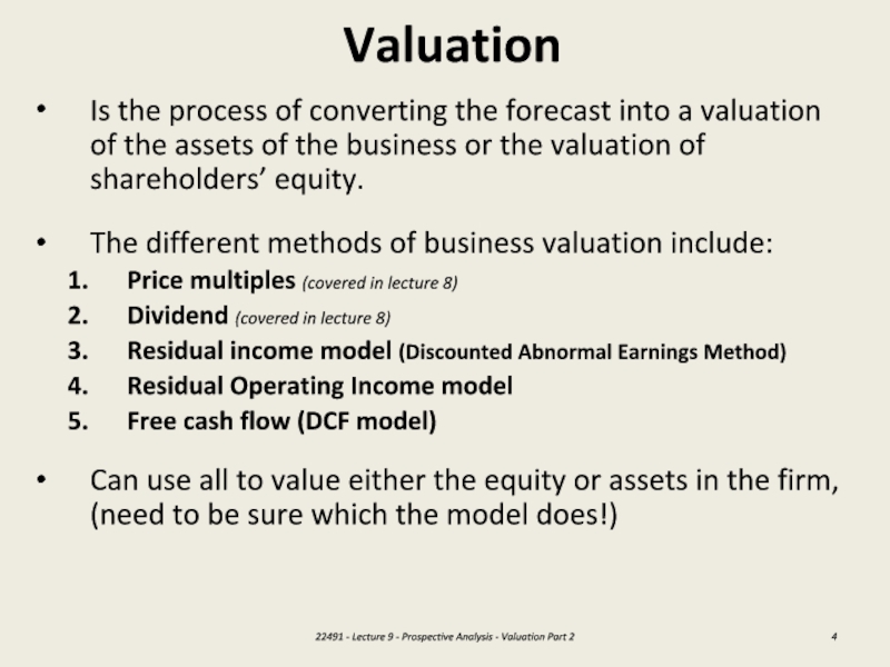
Слайд 4Valuation
Is the process of converting the forecast into a valuation
of the assets of the business or the valuation of
shareholders’ equity.The different methods of business valuation include:
Price multiples (covered in lecture 8)
Dividend (covered in lecture 8)
Residual income model (Discounted Abnormal Earnings Method)
Residual Operating Income model
Free cash flow (DCF model)
Can use all to value either the equity or assets in the firm, (need to be sure which the model does!)
22491 - Lecture 9 - Prospective Analysis - Valuation Part 2
Слайд 5Revision
Last lecture we looked at 2 valuation techniques:
Price multiples
Dividend discount
model
22491 - Lecture 9 - Prospective Analysis - Valuation Part
2Слайд 6Valuation Using Multiples
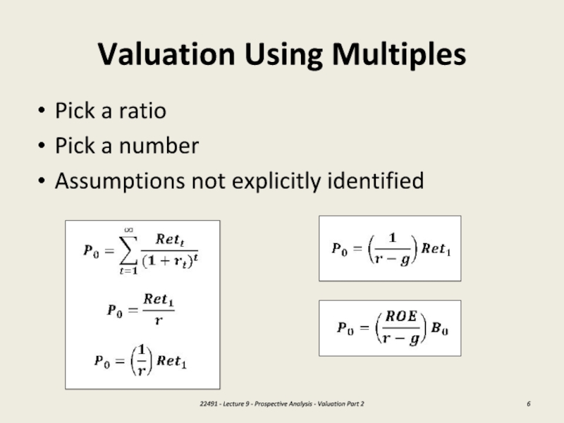
Pick a ratio
Pick a number
Assumptions not
explicitly identified
22491 - Lecture 9 - Prospective Analysis - Valuation
Part 2Слайд 7Discounted Dividend Model
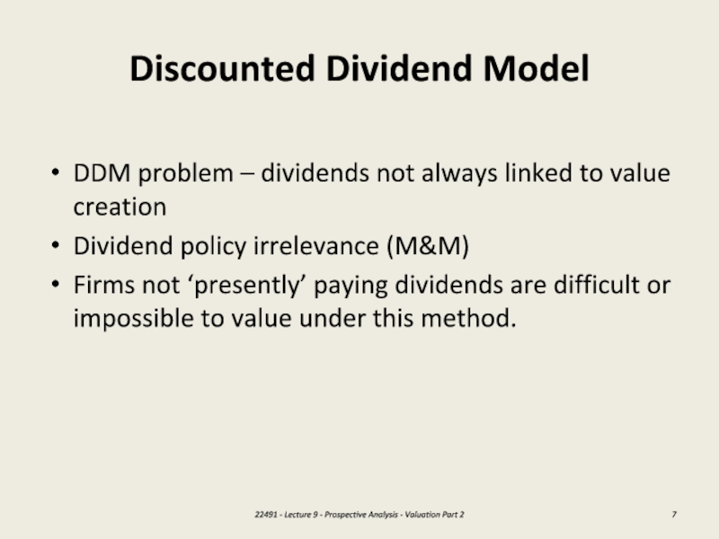
DDM problem – dividends not always linked to
value creation
Dividend policy irrelevance (M&M)
Firms not ‘presently’ paying dividends are
difficult or impossible to value under this method.22491 - Lecture 9 - Prospective Analysis - Valuation Part 2
Слайд 8Earnings
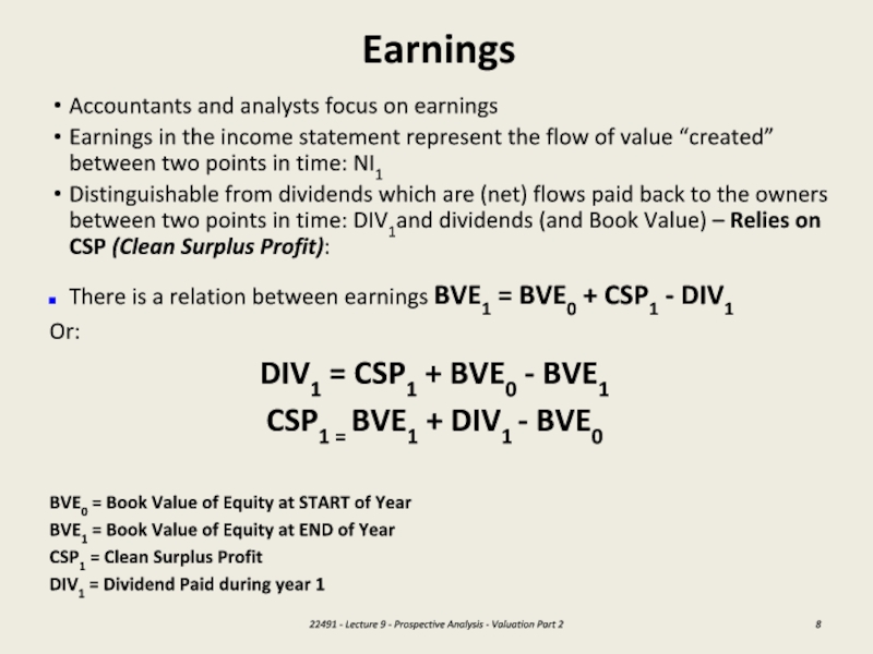
Accountants and analysts focus on earnings
Earnings in the income statement
represent the flow of value “created” between two points in
time: NI1Distinguishable from dividends which are (net) flows paid back to the owners between two points in time: DIV1and dividends (and Book Value) – Relies on CSP (Clean Surplus Profit):
There is a relation between earnings BVE1 = BVE0 + CSP1 - DIV1
Or:
DIV1 = CSP1 + BVE0 - BVE1
CSP1 = BVE1 + DIV1 - BVE0
BVE0 = Book Value of Equity at START of Year
BVE1 = Book Value of Equity at END of Year
CSP1 = Clean Surplus Profit
DIV1 = Dividend Paid during year 1
22491 - Lecture 9 - Prospective Analysis - Valuation Part 2
Слайд 9Residual Income Model
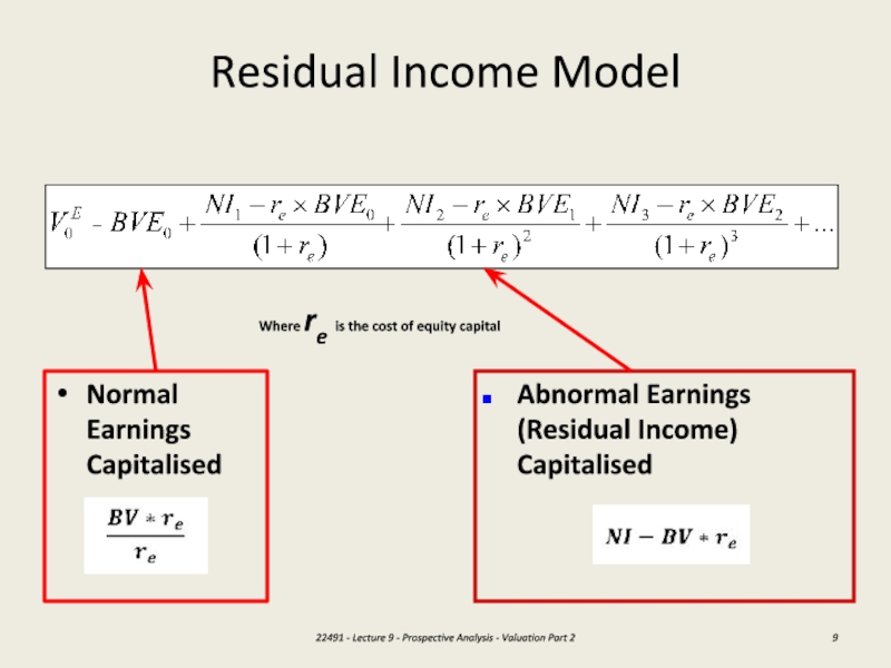
Normal Earnings Capitalised
Abnormal Earnings (Residual Income) Capitalised
22491 -
Lecture 9 - Prospective Analysis - Valuation Part 2
Where re
is the cost of equity capitalСлайд 11Residual Income Model
Requires forecasts to infinity
Can forecast far enough into
the future that residual income approaches zero
Or need a finite
horizon forecast model22491 - Lecture 9 - Prospective Analysis - Valuation Part 2
Слайд 13Residual Income Model – Terminal Values
Choice of 3 simple ways
to calculate a terminal value at some time in the
future – our forecast horizon3 choices:
Residual Income = 0
Residual Income in perpetuity
Residual Income continues in perpetuity, with growth
Choice dependent on what we know of the firm, and therefore our forecasts
22491 - Lecture 9 - Prospective Analysis - Valuation Part 2
Слайд 14Residual Income Model– steps in valuation
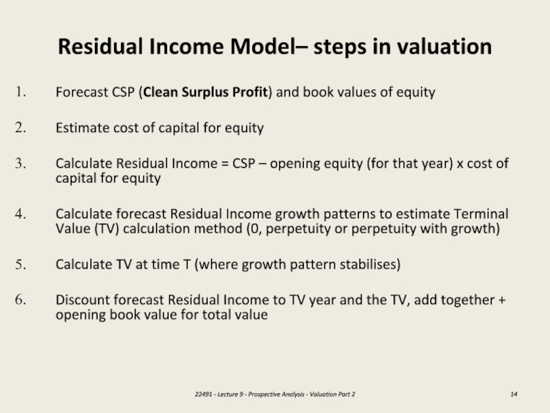
Forecast CSP (Clean Surplus Profit)
and book values of equity
Estimate cost of capital for equity
Calculate
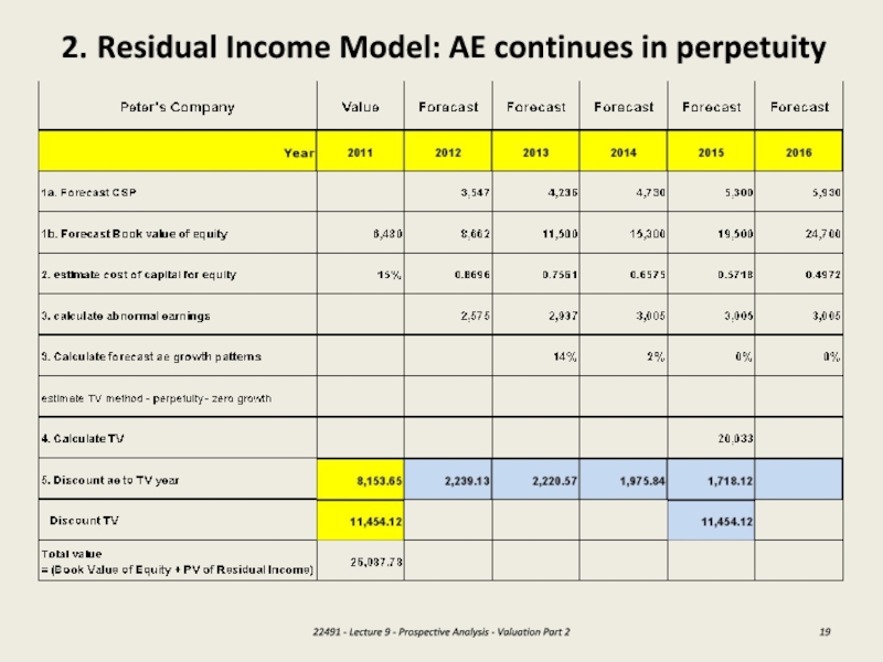
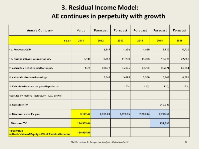
Residual Income = CSP – opening equity (for that year) x cost of capital for equityCalculate forecast Residual Income growth patterns to estimate Terminal Value (TV) calculation method (0, perpetuity or perpetuity with growth)
Calculate TV at time T (where growth pattern stabilises)
Discount forecast Residual Income to TV year and the TV, add together + opening book value for total value
22491 - Lecture 9 - Prospective Analysis - Valuation Part 2
Слайд 151. Residual Income Model: AE = 0
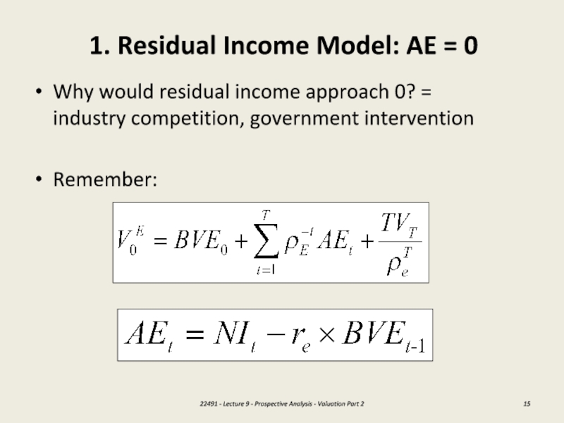
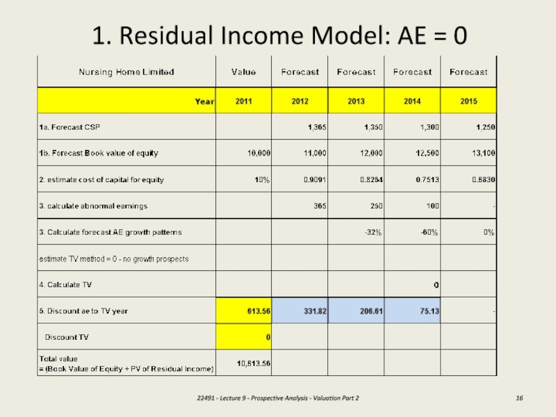
Why would residual income
approach 0? = industry competition, government intervention
Remember:
22491 - Lecture 9
- Prospective Analysis - Valuation Part 2Слайд 182. Residual Income Model:
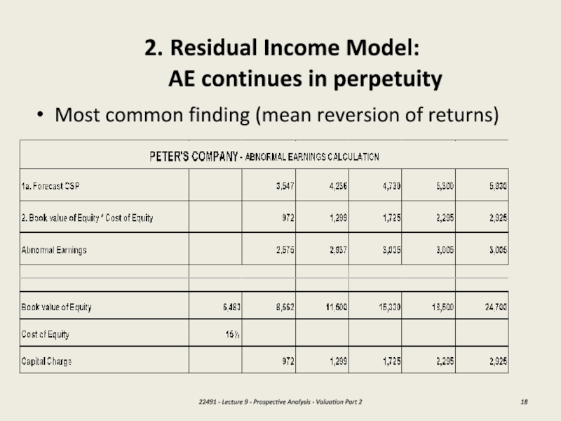
AE continues in perpetuity
Most common finding
(mean reversion of returns)
22491 - Lecture 9 - Prospective Analysis
- Valuation Part 2Слайд 192. Residual Income Model: AE continues in perpetuity
22491 - Lecture
9 - Prospective Analysis - Valuation Part 2
Слайд 203. Residual Income Model:
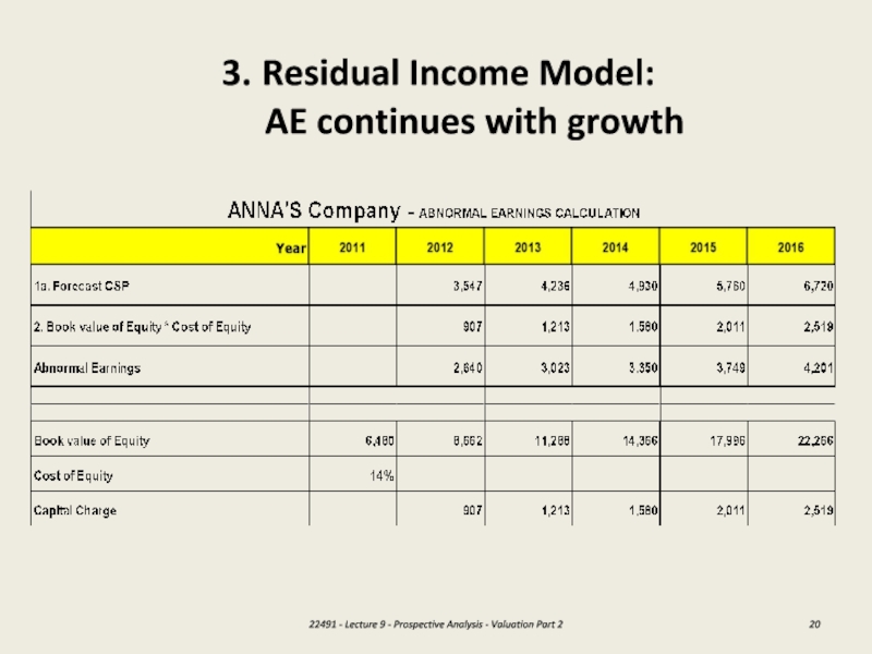
AE continues with growth
22491 - Lecture 9
- Prospective Analysis - Valuation Part 2
Слайд 213. Residual Income Model:
AE continues in perpetuity with growth
22491
- Lecture 9 - Prospective Analysis - Valuation Part 2
Слайд 22Residual Income Model: practice question
Estimate the value of Charles’ company
using the abnormal earnings approach:
22491 - Lecture 9 - Prospective
Analysis - Valuation Part 2Слайд 23Residual Income Model:
practice question – Template solution
22491 - Lecture
9 - Prospective Analysis - Valuation Part 2
Слайд 24Residual Income Model:
practice question – Solution
22491 - Lecture 9
- Prospective Analysis - Valuation Part 2
Слайд 25Residual Income Model
Advantages:
Academic research shows that this method out performs
many of the other models
Focus on value drivers
Profitability of investment
and growth in investmentDirects strategic thinking
Incorporates the financial statements
Incorporates the balance sheet (book value)
Forecasts the income statement and the balance sheet
Uses accrual accounting
Recognizes value added
Matches value added to value lost
Treats investment as an asset
Versatility
Can be used with a wide variety of accounting principles
Aligned with what people forecast
Can be validated
Disadvantages:
Accounting Complexity
Requires understanding of how accounting works
Suspect accounting
Accounting numbers can be suspect
Forecast Horizon
Forecast horizon depends on the quality of the accounting
22491 - Lecture 9 - Prospective Analysis - Valuation Part 2
Слайд 26Residual Operating Income Model
(RIM Modified)
Residual Income Model– uses cost
of capital (equity)
Cost of capital (equity) = changes every time
leverage changes (cost of capital debt)Residual Operating Income Model – uses cost of capital (firm)
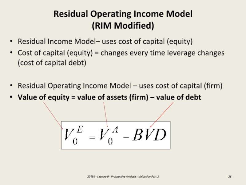
Value of equity = value of assets (firm) – value of debt
22491 - Lecture 9 - Prospective Analysis - Valuation Part 2
Слайд 27Residual Operating Income Model
Therefore - can also estimate equity values
by calculating the value of assets and subtracting the book
value of debt (often simpler – no need to think about leverage)Value of Equity = Value of Assets – Book Value of Debt
Question: So how to value the assets (firm)?
Equity = NOA – Net debt (NFL)
CSP = NOPAT – Net financing expenses
NOA = Net Operating Assets
CSP = Clean Surplus Profit
Net Debt = Net Financial Liabilities = Interest Bearing Debt (Current + Non Current) – (Cash +Cash Equivalents)
NOPAT = Net Operating Profit after tax
Net Financing Expense = Interest Expense – Interest Revenue
22491 - Lecture 9 - Prospective Analysis - Valuation Part 2
Слайд 28Residual OPERATING Income Model
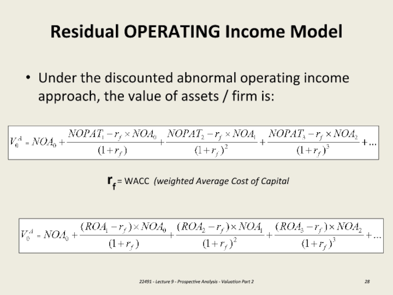
Under the discounted abnormal operating income approach,
the value of assets / firm is:
22491 - Lecture 9
- Prospective Analysis - Valuation Part 2rf = WACC (weighted Average Cost of Capital
Слайд 29Residual Operating Income Model
Gives the same result as abnormal earnings
valuation (as long as cost of capital for equity is
adjusted each time leverage changes)22491 - Lecture 9 - Prospective Analysis - Valuation Part 2
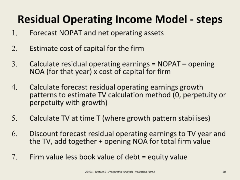
Слайд 30Residual Operating Income Model - steps
Forecast NOPAT and net operating
assets
Estimate cost of capital for the firm
Calculate residual operating earnings
= NOPAT – opening NOA (for that year) x cost of capital for firmCalculate forecast residual operating earnings growth patterns to estimate TV calculation method (0, perpetuity or perpetuity with growth)
Calculate TV at time T (where growth pattern stabilises)
Discount forecast residual operating earnings to TV year and the TV, add together + opening NOA for total firm value
Firm value less book value of debt = equity value
22491 - Lecture 9 - Prospective Analysis - Valuation Part 2
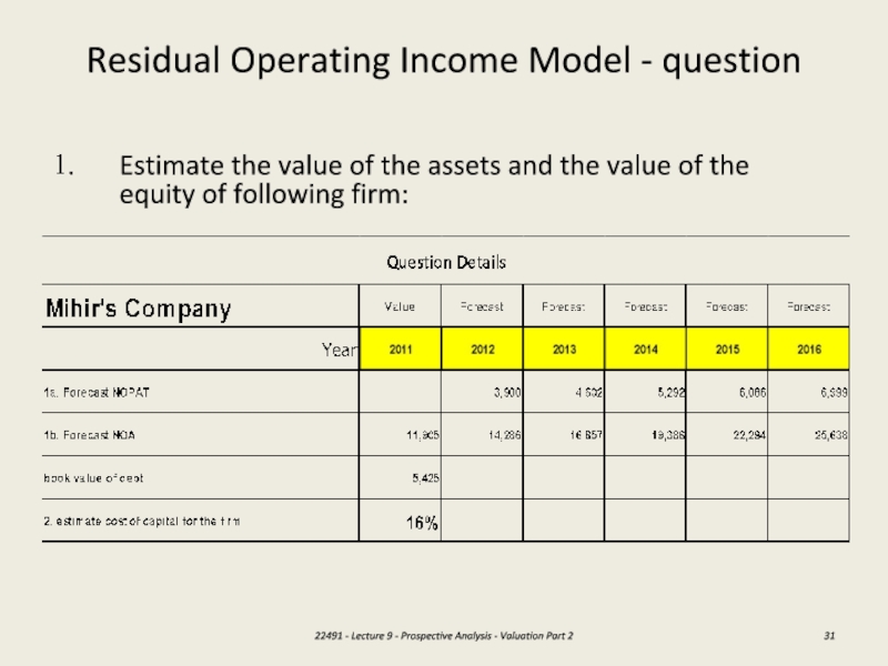
Слайд 31Residual Operating Income Model - question
Estimate the value of the
assets and the value of the equity of following firm:
22491
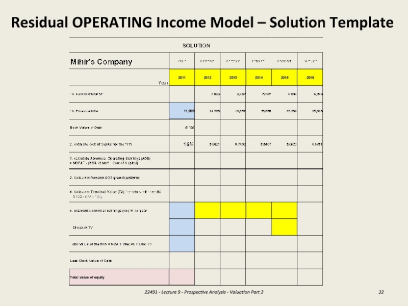
- Lecture 9 - Prospective Analysis - Valuation Part 2Слайд 32Residual OPERATING Income Model – Solution Template
22491 - Lecture 9
- Prospective Analysis - Valuation Part 2
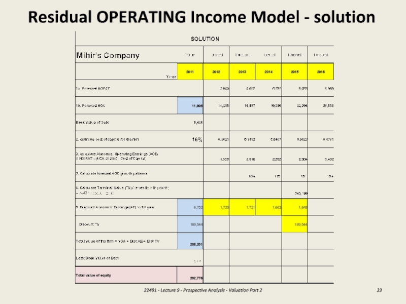
Слайд 33Residual OPERATING Income Model - solution
22491 - Lecture 9 -
Prospective Analysis - Valuation Part 2
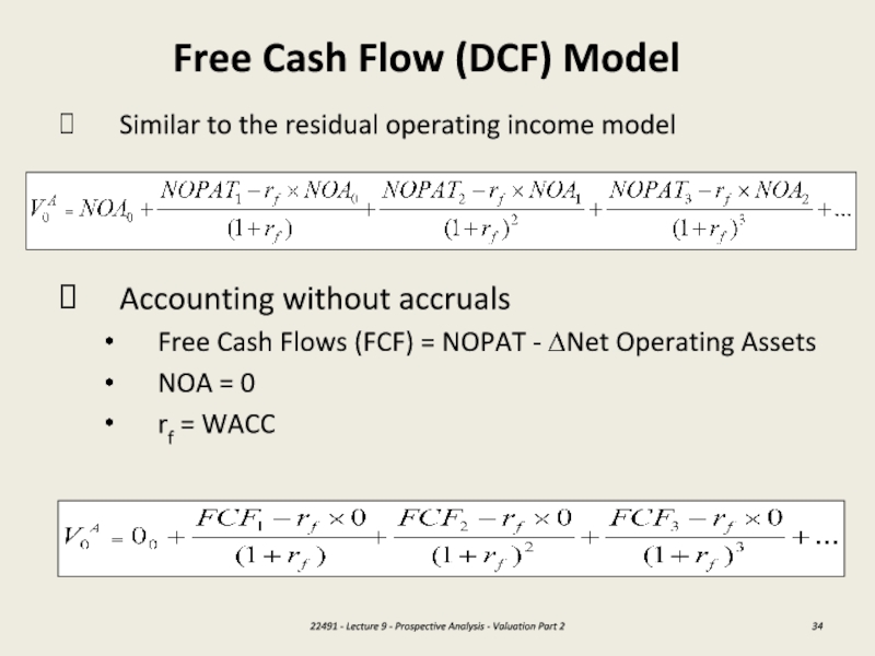
Слайд 34Free Cash Flow (DCF) Model
Similar to the residual operating income
model
Accounting without accruals
Free Cash Flows (FCF) = NOPAT - ∆Net
Operating AssetsNOA = 0
rf = WACC
22491 - Lecture 9 - Prospective Analysis - Valuation Part 2
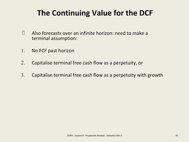
Слайд 35Also forecasts over an infinite horizon: need to make a
terminal assumption:
No FCF past horizon
Capitalise terminal free cash flow as
a perpetuity, orCapitalise terminal free cash flow as a perpetuity with growth
The Continuing Value for the DCF
22491 - Lecture 9 - Prospective Analysis - Valuation Part 2
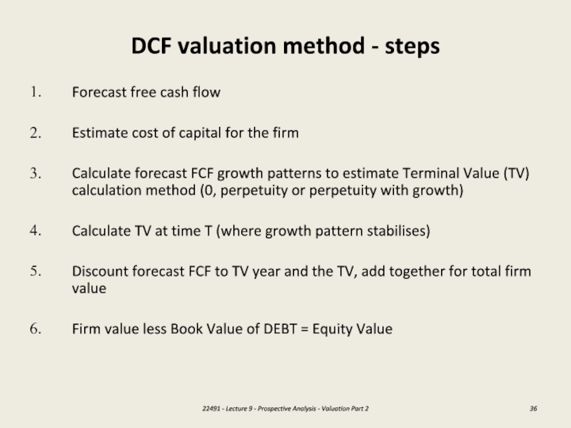
Слайд 36DCF valuation method - steps
Forecast free cash flow
Estimate cost of
capital for the firm
Calculate forecast FCF growth patterns to estimate
Terminal Value (TV) calculation method (0, perpetuity or perpetuity with growth)Calculate TV at time T (where growth pattern stabilises)
Discount forecast FCF to TV year and the TV, add together for total firm value
Firm value less Book Value of DEBT = Equity Value
22491 - Lecture 9 - Prospective Analysis - Valuation Part 2
Слайд 40What are the problems with DCF?
Cash flow from operations (value
added) is reduced by investments (which also add value): investments
are treated as value lossesValue received is not matched against value surrendered to generate value - except for long forecast horizons
Note: analysts forecast earnings, not cash flows
22491 - Lecture 9 - Prospective Analysis - Valuation Part 2
Слайд 41DCF Analysis
Advantages
Easy concept: cash flows are “real” and easy to think
about; they are not
affected by accounting rules
Familiarity:
is a straight application of familiar net present valuetechniques
Disadvantages
Suspect concept: → free cash flow does not measure value added in the
short run; value gained is not matched with value given up
→ free cash flow fails to recognize value generated that
does not involve cash flows
→ investment is treated as a loss of value
→ free cash flow is partly a liquidation concept; firms
increase free cash flow by cutting back on investments
Forecast horizons: can require long forecast horizons to recognize cash
inflows from investments, particularly when investments
are growing
Validation: it is hard to validate free cash flow forecasts
Not aligned with
what people
forecast: analysts forecast earnings, not free cash flow; adjusting
earnings forecasts to free cash forecasts requires further
forecasting of accruals
When It Works Best
When the investment pattern is such as to produce constant free cash flow or free cash flow growing at a constant rate
22491 - Lecture 9 - Prospective Analysis - Valuation Part 2
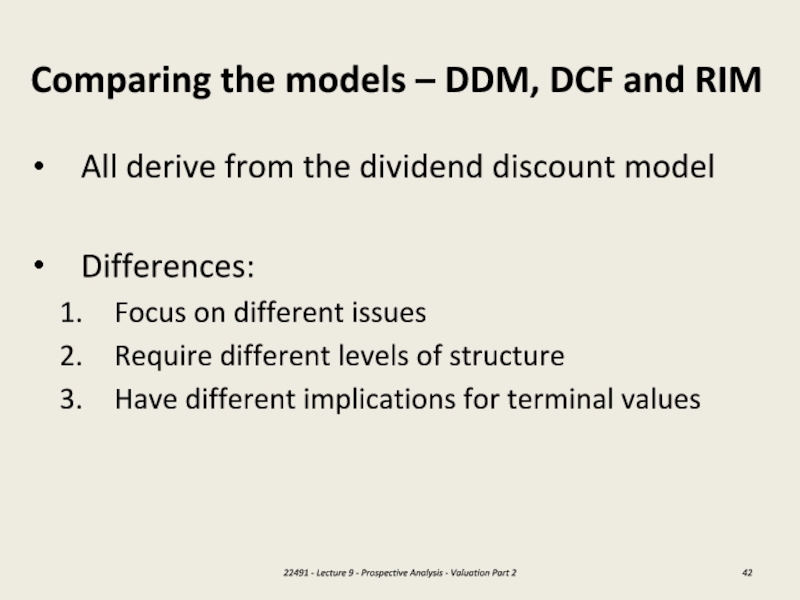
Слайд 42Comparing the models – DDM, DCF and RIM
All derive from
the dividend discount model
Differences:
Focus on different issues
Require different levels of
structureHave different implications for terminal values
22491 - Lecture 9 - Prospective Analysis - Valuation Part 2
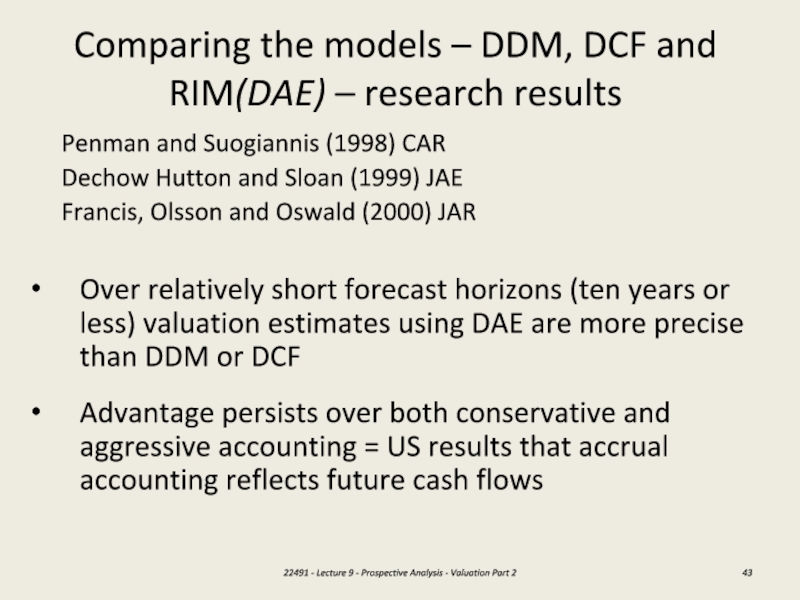
Слайд 43Comparing the models – DDM, DCF and RIM(DAE) – research
results
Penman and Suogiannis (1998) CAR
Dechow Hutton and Sloan (1999) JAE
Francis,
Olsson and Oswald (2000) JAROver relatively short forecast horizons (ten years or less) valuation estimates using DAE are more precise than DDM or DCF
Advantage persists over both conservative and aggressive accounting = US results that accrual accounting reflects future cash flows
22491 - Lecture 9 - Prospective Analysis - Valuation Part 2
Слайд 44Summary
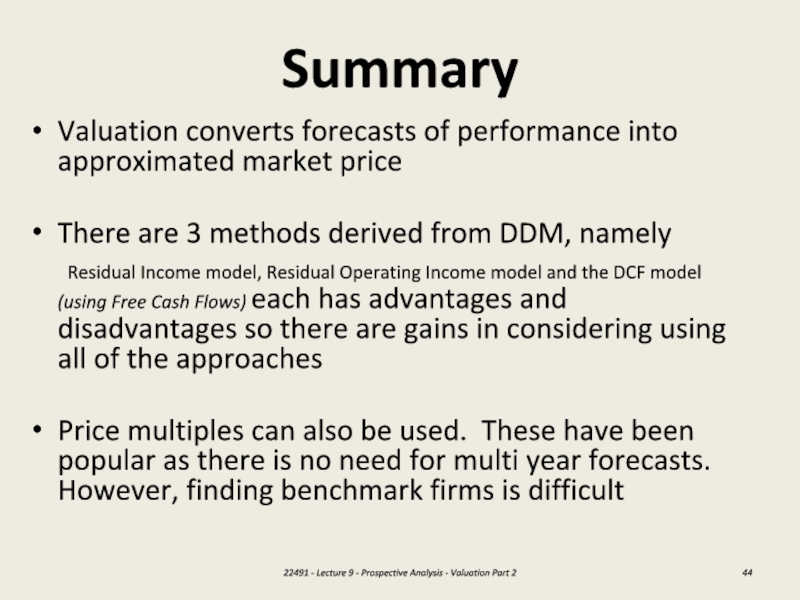
Valuation converts forecasts of performance into approximated market price
There are
3 methods derived from DDM, namely
Residual Income model, Residual
Operating Income model and the DCF model (using Free Cash Flows) each has advantages and disadvantages so there are gains in considering using all of the approachesPrice multiples can also be used. These have been popular as there is no need for multi year forecasts. However, finding benchmark firms is difficult
22491 - Lecture 9 - Prospective Analysis - Valuation Part 2
