Разделы презентаций
- Разное
- Английский язык
- Астрономия
- Алгебра
- Биология
- География
- Геометрия
- Детские презентации
- Информатика
- История
- Литература
- Математика
- Медицина
- Менеджмент
- Музыка
- МХК
- Немецкий язык
- ОБЖ
- Обществознание
- Окружающий мир
- Педагогика
- Русский язык
- Технология
- Физика
- Философия
- Химия
- Шаблоны, картинки для презентаций
- Экология
- Экономика
- Юриспруденция
machine_learning _ lecture 4_2
Содержание
- 1. machine_learning _ lecture 4_2
- 2. Lecture 4.2 Linear Regression. Linear Regression with Gradient Descent. Regularization
- 3. https://www.youtube.com/watch?v=vMh0zPT0tLIhttps://www.youtube.com/watch?v=Q81RR3yKn30https://www.youtube.com/watch?v=NGf0voTMlcshttps://www.youtube.com/watch?v=1dKRdX9bfIo
- 4. Gradient descent is a method of numerical
- 5. Gradient Descent is the most common optimization algorithm
- 6. Слайд 6
- 7. Слайд 7
- 8. Linear Regression in Python using gradient descent
- 9. For many machine learning problems with a
- 10. Regularization: Ridge, Lasso and Elastic Net Models
- 11. Lasso Regression Basics Lasso performs a so
- 12. Ordinary least squares (OLS)
- 13. Слайд 13
- 14. The LASSO minimizes the sum of squared
- 15. Parameter In practice, the tuning parameter
- 16. This additional term penalizes the model for
- 17. Lasso Regression with Python
- 18. Ridge regressionRidge regression also adds an additional
- 19. rr = Ridge(alpha=0.01)rr.fit(X_train, y_train)
- 20. Elastic Net Elastic Net includes both L-1
- 21. the elastic net adds a quadratic part
- 22. #Elastic Netmodel_enet = ElasticNet(alpha = 0.01)model_enet.fit(X_train, y_train)
- 23. Lecture for Home workhttp://subtitlelist.com/en/Lecture-25-%E2%80%94-Linear-Regression-With-One-Variable-Gradient-Descent-%E2%80%94-Andrew-Ng-10360
- 24. Скачать презентанцию
Lecture 4.2 Linear Regression. Linear Regression with Gradient Descent. Regularization
Слайды и текст этой презентации
Слайд 3
https://www.youtube.com/watch?v=vMh0zPT0tLI
https://www.youtube.com/watch?v=Q81RR3yKn30
https://www.youtube.com/watch?v=NGf0voTMlcs
https://www.youtube.com/watch?v=1dKRdX9bfIo
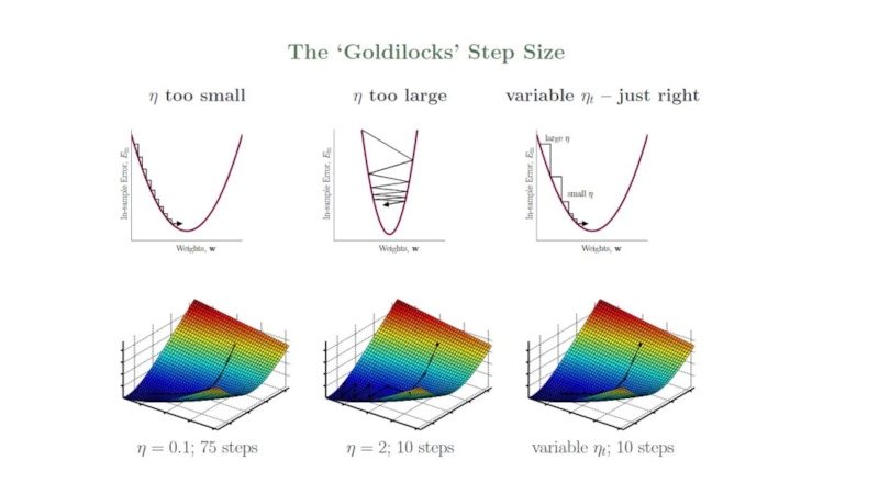
Слайд 5Gradient Descent is the most common optimization algorithm in machine learning and deep learning.
It is a first-order optimization algorithm. This means it only
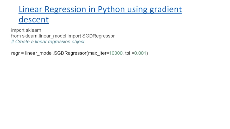
takes into account the first derivative when performing the updates on the parameters. On each iteration, we update the parameters in the opposite direction of the gradient of the objective function J(w) w.r.t the parameters where the gradient gives the direction of the steepest ascent. The size of the step we take on each iteration to reach the local minimum is determined by the learning rate α. Therefore, we follow the direction of the slope downhill until we reach a local minimum.Слайд 8Linear Regression in Python using gradient descent
import sklearn
from sklearn.linear_model import
SGDRegressor
# Create a linear regression object
regr = linear_model.SGDRegressor(max_iter=10000, tol
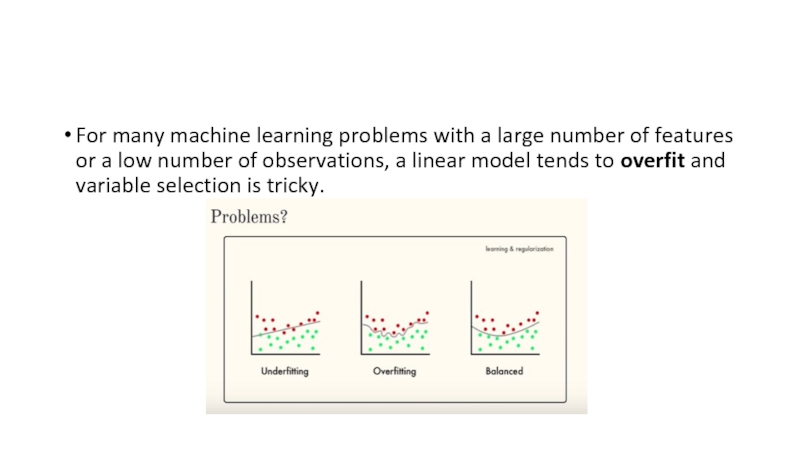
=0.001) Слайд 9For many machine learning problems with a large number of
features or a low number of observations, a linear model
tends to overfit and variable selection is tricky.Слайд 10Regularization: Ridge, Lasso and Elastic Net
Models that use shrinkage such as Lasso
and Ridge can improve the prediction accuracy as they reduce
the estimation variance while providing an interpretable final model.In this tutorial, we will examine Ridge and Lasso regressions, compare it to the classical linear regression and apply it to a dataset in Python. Ridge and Lasso build on the linear model, but their fundamental peculiarity is regularization. The goal of these methods is to improve the loss function so that it depends not only on the sum of the squared differences but also on the regression coefficients.
One of the main problems in the construction of such models is the correct selection of the regularization parameter. Сomparing to linear regression, Ridge and Lasso models are more resistant to outliers and the spread of data. Overall, their main purpose is to prevent overfitting.
The main difference between Ridge regression and Lasso is how they assign a penalty term to the coefficients.
Слайд 11Lasso Regression Basics
Lasso performs a so called L1 regularization (a
process of introducing additional information in order to prevent overfitting),
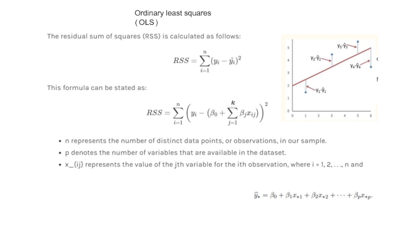
i.e. adds penalty equivalent to absolute value of the magnitude of coefficients.In particular, the minimization objective does not only include the residual sum of squares (RSS) - like in the OLS regression setting - but also the sum of the absolute value of coefficients.
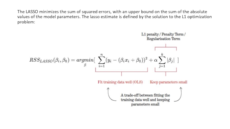
Слайд 14The LASSO minimizes the sum of squared errors, with an
upper bound on the sum of the absolute values of
the model parameters. The lasso estimate is defined by the solution to the L1 optimization problem:Слайд 15Parameter
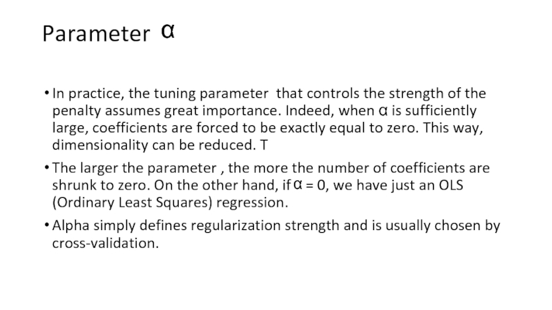
In practice, the tuning parameter that controls the strength
of the penalty assumes great importance. Indeed, when α is
sufficiently large, coefficients are forced to be exactly equal to zero. This way, dimensionality can be reduced. TThe larger the parameter , the more the number of coefficients are shrunk to zero. On the other hand, if = 0, we have just an OLS (Ordinary Least Squares) regression.
Alpha simply defines regularization strength and is usually chosen by cross-validation.
α
α
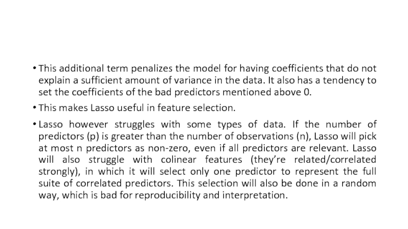
Слайд 16This additional term penalizes the model for having coefficients that
do not explain a sufficient amount of variance in the
data. It also has a tendency to set the coefficients of the bad predictors mentioned above 0.This makes Lasso useful in feature selection.
Lasso however struggles with some types of data. If the number of predictors (p) is greater than the number of observations (n), Lasso will pick at most n predictors as non-zero, even if all predictors are relevant. Lasso will also struggle with colinear features (they’re related/correlated strongly), in which it will select only one predictor to represent the full suite of correlated predictors. This selection will also be done in a random way, which is bad for reproducibility and interpretation.
Слайд 18Ridge regression
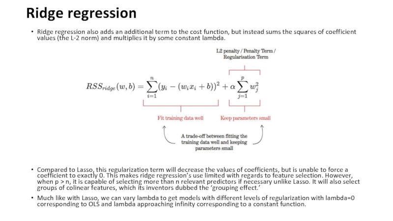
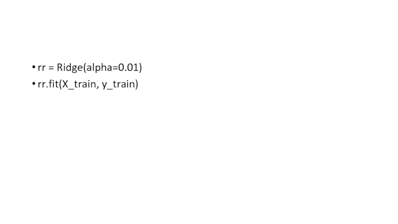
Ridge regression also adds an additional term to the
cost function, but instead sums the squares of coefficient values
(the L-2 norm) and multiplies it by some constant lambda.Compared to Lasso, this regularization term will decrease the values of coefficients, but is unable to force a coefficient to exactly 0. This makes ridge regression’s use limited with regards to feature selection. However, when p > n, it is capable of selecting more than n relevant predictors if necessary unlike Lasso. It will also select groups of colinear features, which its inventors dubbed the ‘grouping effect.’
Much like with Lasso, we can vary lambda to get models with different levels of regularization with lambda=0 corresponding to OLS and lambda approaching infinity corresponding to a constant function.
Слайд 20Elastic Net
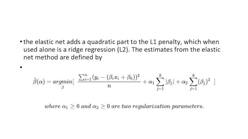
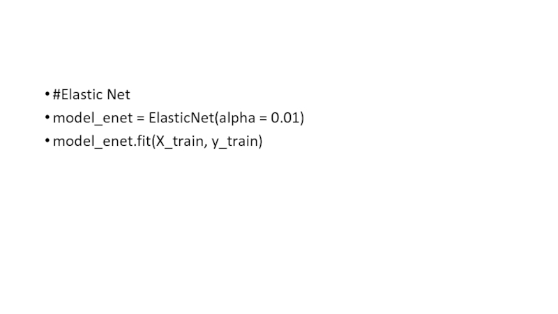
Elastic Net includes both L-1 and L-2 norm regularization
terms.
This gives us the benefits of both Lasso and
Ridge regression.It has been found to have predictive power better than Lasso, while still performing feature selection.
We therefore get the best of both worlds, performing feature selection of Lasso with the feature-group selection of Ridge.


